Advanced Workflows for High-Level Users • betaregscale

Audience and scope

This vignette is designed for analysts who are already familiar with beta regression and require a production-oriented workflow featuring:

reproducible model selection;
inferential and predictive diagnostics;
mixed-effects escalation (brs -> brsmm) with Likelihood Ratio (LR) comparisons;
high-signal reporting tables for technical decision-making.

library(betaregscale)

1) Reproducible simulation and data checks

n <- 150
d <- data.frame(
  x1 = rnorm(n),
  x2 = rnorm(n),
  z1 = rnorm(n)
)

sim <- brs_sim(
  formula = ~ x1 + x2 | z1,
  data = d,
  beta = c(0.15, 0.55, -0.30),
  zeta = c(-0.10, 0.35),
  link = "logit",
  link_phi = "logit",
  ncuts = 100,
  repar = 2
)

kbl10(head(sim, 10))

left	right	yt	y	delta	x1	x2	z1
0.905	0.915	0.91	91	3	0.5206	0.0243	-0.1486
0.005	0.015	0.01	1	3	-1.0797	0.3346	-0.1830
0.315	0.325	0.32	32	3	0.1392	0.9894	-0.8581
0.425	0.435	0.43	43	3	-0.0847	0.5004	0.9582
0.005	0.015	0.01	1	3	-0.6666	0.5769	-0.8391
0.000	0.005	0.00	0	1	-2.5161	1.1427	-0.7597
0.185	0.195	0.19	19	3	-0.7351	-0.7074	-0.8665
0.095	0.105	0.10	10	3	-1.0201	-0.6186	1.6590
0.995	1.000	1.00	100	2	0.1136	-0.0083	0.5569
0.165	0.175	0.17	17	3	-0.4738	0.3389	0.6014

kbl10(
  data.frame(
    n = nrow(sim),
    exact = sum(sim$delta == 0),
    left = sum(sim$delta == 1),
    right = sum(sim$delta == 2),
    interval = sum(sim$delta == 3)
  ),
  digits = 4
)

n	exact	left	right	interval
150	0	9	10	131

brs_sim() coarsens each draw exactly as the likelihood assumes, so the censoring is non-informative. Its delta argument can force one type on every row; delta = 1 or 2 censors each row at the cell of its own score, which is informative censoring with no finite MLE, and brs_sim() warns. Leave delta = NULL for studies of the estimator.

2) Fixed-effects candidate set and model ranking

fit_logit <- brs(y ~ x1 + x2 | z1, data = sim, link = "logit", repar = 2)
fit_probit <- brs(y ~ x1 + x2 | z1, data = sim, link = "probit", repar = 2)
fit_cauchit <- brs(y ~ x1 + x2 | z1, data = sim, link = "cauchit", repar = 2)

tab_rank <- brs_table(
  logit = fit_logit,
  probit = fit_probit,
  cauchit = fit_cauchit
)
kbl10(tab_rank)

model	nobs	npar	logLik	AIC	BIC	pseudo_r2	left	right	interval	prop_left	prop_right	prop_interval
logit	150	5	-632.6093	1275.219	1290.272	0.2075	9	10	131	0.06	0.0667	0.8733
probit	150	5	-632.4476	1274.895	1289.948	0.2095	9	10	131	0.06	0.0667	0.8733
cauchit	150	5	-633.4406	1276.881	1291.934	0.1334	9	10	131	0.06	0.0667	0.8733

3) Inference stack: Wald + bootstrap + AME

kbl10(brs_est(fit_logit))

variable	estimate	se	z_value	p_value	ci_lower	ci_upper
(Intercept)	0.0880	0.1059	0.8306	0.4062	-0.1196	0.2956
x1	0.6022	0.1051	5.7325	0.0000	0.3963	0.8081
x2	-0.3393	0.1240	-2.7371	0.0062	-0.5823	-0.0963
(phi)_(Intercept)	-0.0823	0.1016	-0.8099	0.4180	-0.2814	0.1168
(phi)_z1	0.2621	0.0955	2.7447	0.0061	0.0749	0.4493

kbl10(confint(fit_logit))

	2.5 %	97.5 %
(Intercept)	-0.1196	0.2956
x1	0.3963	0.8081
x2	-0.5823	-0.0963
(phi)_(Intercept)	-0.2814	0.1168
(phi)_z1	0.0749	0.4493


# Draws are kept so that the plots below can reuse this single fit rather
# than resampling a second time.
boot_tab <- brs_bootstrap(fit_logit, R = 30, level = 0.95, keep_draws = TRUE)
kbl10(head(boot_tab, 10))

parameter	estimate	se_boot	ci_lower	ci_upper	mcse_lower	mcse_upper	wald_lower	wald_upper	level
(Intercept)	0.0880	0.1056	-0.0375	0.3209	0.0159	0.0409	-0.1196	0.2956	0.95
x1	0.6022	0.1138	0.3534	0.7741	0.0529	0.0278	0.3963	0.8081	0.95
x2	-0.3393	0.1348	-0.5710	-0.1492	0.0224	0.0210	-0.5823	-0.0963	0.95
(phi)_(Intercept)	-0.0823	0.1035	-0.2708	0.0564	0.0209	0.0156	-0.2814	0.1168	0.95
(phi)_z1	0.2621	0.1028	0.1054	0.4761	0.0180	0.0334	0.0749	0.4493	0.95


set.seed(2026) # For marginal effects simulation
ame_mu <- brs_marginaleffects(
  fit_logit,
  model = "mean",
  type = "response",
  interval = TRUE,
  n_sim = 60,
  keep_draws = TRUE
)
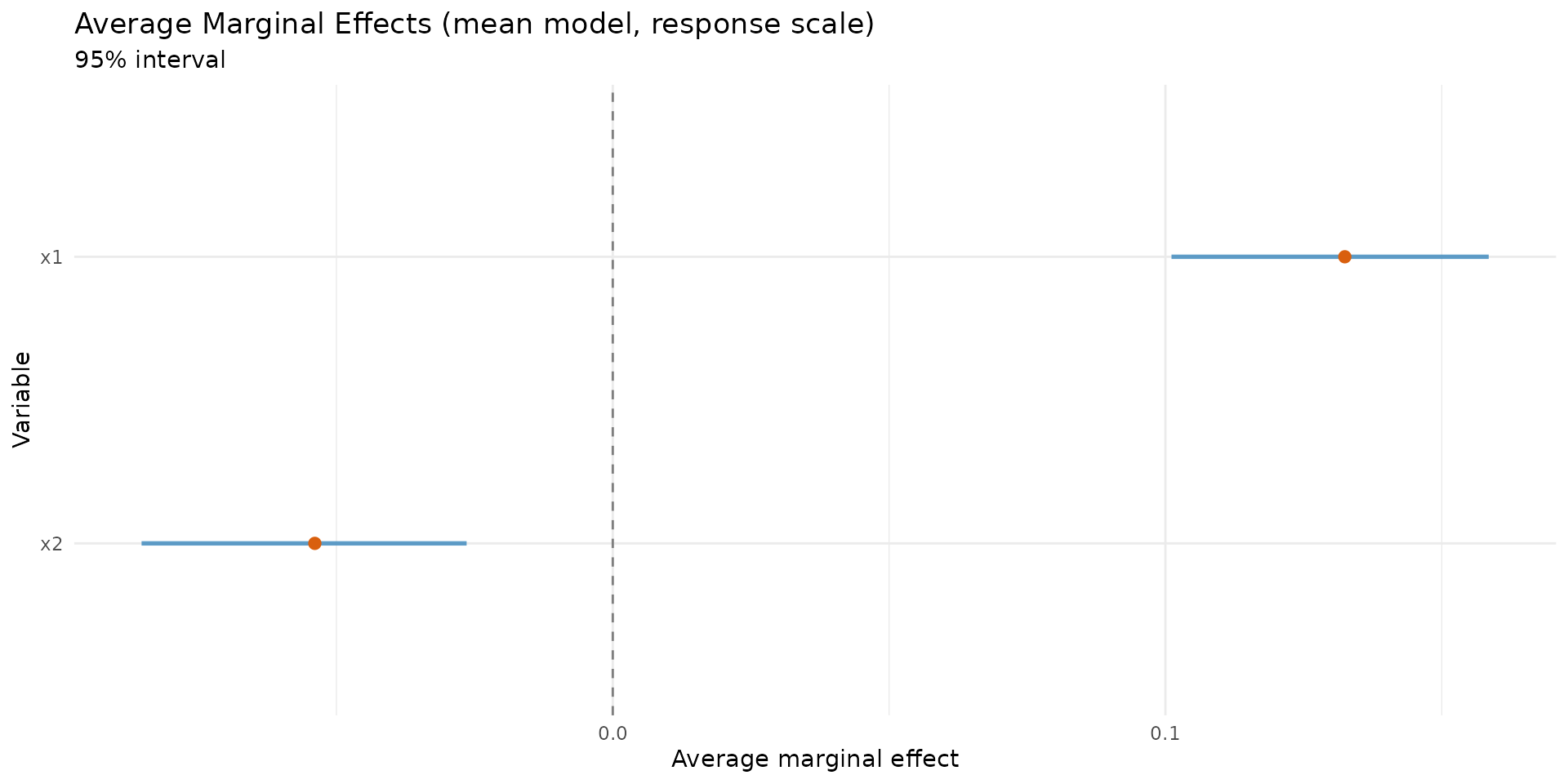
kbl10(ame_mu)

variable	ame	std.error	ci.lower	ci.upper	model	type	n
x1	0.1366	0.0221	0.0964	0.176	mean	response	150
x2	-0.0770	0.0248	-0.1196	-0.020	mean	response	150

Each bootstrap replicate draws a new response at the fitted shapes and refits the original formula on a copy of the data, so factors, transformations and prepared data keep their structure; each row keeps its observation mechanism (exact, score, or analyst thresholds, which are treated as fixed and non-informative). Refits start from the fitted estimate and use the compiled Hessian. Failed replicates are counted in the printed header. ci_type = "bca" is also available: with parametric resampling and a leave-one-out jackknife it is an approximation (a warning says so once per session) and costs R + n fits instead of R; see ?brs_bootstrap.

if (requireNamespace("ggplot2", quietly = TRUE)) {
  autoplot.brs_bootstrap(
    boot_tab,
    type = "ci_forest",
    title = "Bootstrap (percentile) vs Wald intervals"
  )
  autoplot.brs_marginaleffects(ame_mu, type = "forest")
}

4) Prediction layer on analyst scale

score_prob <- brs_predict_scoreprob(fit_logit, scores = 0:10)
kbl10(score_prob[1:8, 1:7])

score_0	score_1	score_2	score_3	score_4	score_5	score_6
0.0150	0.0166	0.0131	0.0115	0.0105	0.0098	0.0093
0.1131	0.0595	0.0376	0.0292	0.0244	0.0213	0.0191
0.0292	0.0288	0.0219	0.0188	0.0169	0.0156	0.0146
0.0793	0.0432	0.0276	0.0216	0.0182	0.0160	0.0144
0.0610	0.0456	0.0317	0.0259	0.0225	0.0201	0.0184
0.3873	0.0875	0.0471	0.0335	0.0264	0.0219	0.0189
0.0260	0.0267	0.0206	0.0178	0.0161	0.0149	0.0140
0.1375	0.0532	0.0315	0.0236	0.0194	0.0166	0.0147

5) Out-of-sample validation

set.seed(2026) # For cross-validation reproducibility
cv_tab <- brs_cv(
  y ~ x1 + x2 | z1,
  data = sim,
  k = 5,
  repeats = 2,
  repar = 2
)
kbl10(head(cv_tab, 10))

repeat	fold	n_train	n_test	log_score	rmse_yt	mae_yt	converged	error
1	1	120	30	-4.1078	0.3298	0.2945	TRUE	NA
1	2	120	30	-4.4249	0.3907	0.3447	TRUE	NA
1	3	120	30	-4.0241	0.3290	0.2950	TRUE	NA
1	4	120	30	-4.4575	0.3378	0.2984	TRUE	NA
1	5	120	30	-4.2346	0.3401	0.2993	TRUE	NA
2	1	120	30	-4.4746	0.3608	0.3105	TRUE	NA
2	2	120	30	-4.3551	0.3507	0.3146	TRUE	NA
2	3	120	30	-4.1657	0.3262	0.2917	TRUE	NA
2	4	120	30	-3.9674	0.3667	0.3343	TRUE	NA
2	5	120	30	-4.4196	0.3247	0.2831	TRUE	NA

6) Escalation to mixed models

6.1 Simulate clustered data with random intercept + slope

g <- 10
ni <- 25
id <- factor(rep(seq_len(g), each = ni))
n_mm <- length(id)
x1 <- rnorm(n_mm)
x2 <- rbinom(n_mm, size = 1, prob = 1 / 2)

b0 <- rnorm(g, sd = 0.40)
b1 <- rnorm(g, sd = 0.22)

eta_mu <- 0.20 + 0.65 * x1 - 0.30 * x2 + b0[id] + b1[id] * x1
eta_phi <- rep(-0.20, n_mm)

mu <- plogis(eta_mu)
phi <- plogis(eta_phi)
shp <- brs_repar(mu = mu, phi = phi, repar = 2)
y <- round(stats::rbeta(n_mm, shp$shape1, shp$shape2) * 100)

dmm <- data.frame(y = y, id = id, x1 = x1, x2 = x2)
kbl10(head(dmm, 10))

y	id	x1	x2
8	1	-0.5886	0
89	1	-0.2773	1
9	1	-1.6193	0
61	1	-0.1864	1
78	1	-0.5432	1
77	1	-0.3511	1
100	1	0.7576	1
53	1	-0.3713	1
0	1	-0.4505	1
26	1	-0.1020	1

6.2 Fit evolutionary sequence

fit_brs <- brs(y ~ x1 + x2, data = dmm, repar = 2)
fit_ri <- brsmm(y ~ x1 + x2, random = ~ 1 | id, data = dmm, repar = 2)
fit_rs <- brsmm(y ~ x1 + x2, random = ~ 1 + x1 | id, data = dmm, repar = 2)

tab_lr <- anova(fit_brs, fit_ri, fit_rs, test = "Chisq")
tab_lr
#> Likelihood-ratio comparison of brs/brsmm models
#> Rows M2, M3: one added random effect (variance on the boundary); Pr(>Chisq) from the chi-bar-square mixture 1/2 chi2(Df - 1) + 1/2 chi2(Df).
#> 
#>            Df  logLik    AIC    BIC  Chisq Chi Df Pr(>Chisq)   
#> M1 (brs)    4 -1057.0 2122.1 2136.1                            
#> M2 (brsmm)  5 -1054.1 2118.2 2135.8 5.8355      1   0.007853 **
#> M3 (brsmm)  7 -1052.2 2118.3 2143.0 3.8718      2   0.096701 . 
#> ---
#> Signif. codes:  0 '***' 0.001 '**' 0.01 '*' 0.05 '.' 0.1 ' ' 1

6.3 Model choice by LLR/LRT (ANOVA)

The anova() methods provide a practical Likelihood Ratio Test (LLR) workflow:

M0 = brs (no random effects);
M1 = brsmm with random intercept (~ 1 | id);
M2 = brsmm with random intercept + slope (~ 1 + x1 | id).

In nested comparisons, the test statistic is: $LR=2\{\ell(\hat\theta_{\text{complex}})-\ell(\hat\theta_{\text{simple}})\}$

Both steps add one random-effect term whose variance is on the boundary of the parameter space under $H_0$ ( $\sigma^2=0$ ). The reference distribution is then the mixture $\frac12\chi^2_{d-1}+\frac12\chi^2_{d}$ (Self and Liang, 1987; Stram and Lee, 1994): $\frac12\chi^2_0+\frac12\chi^2_1$ for M0 -> M1 and $\frac12\chi^2_1+\frac12\chi^2_2$ for M1 -> M2, where the slope adds a variance and a covariance. anova() uses it for such rows and says so in its heading; the naive $\chi^2_d$ p-value would be too large. A term that adds almost nothing to the likelihood is also flagged by brsmm() (“Variance component at the boundary”).

tab_lr_df <- data.frame(model = rownames(tab_lr), tab_lr, row.names = NULL)
tab_lr_df$decision <- c(
  "baseline",
  ifelse(is.na(tab_lr_df$`Pr(>Chisq)`[2]), "inspect AIC/BIC + diagnostics",
    ifelse(tab_lr_df$`Pr(>Chisq)`[2] < 0.05, "prefer M1 over M0", "prefer M0 (parsimony)")
  ),
  ifelse(is.na(tab_lr_df$`Pr(>Chisq)`[3]), "inspect AIC/BIC + diagnostics",
    ifelse(tab_lr_df$`Pr(>Chisq)`[3] < 0.05, "prefer M2 over M1", "prefer M1 (parsimony)")
  )
)
kbl10(tab_lr_df)

model	Df	logLik	AIC	BIC	Chisq	Chi.Df	Pr..Chisq.	decision
M1 (brs)	4	-1057.029	2122.058	2136.144	NA	NA	NA	baseline
M2 (brsmm)	5	-1054.111	2118.223	2135.830	5.8355	1	0.0079	baseline
M3 (brsmm)	7	-1052.176	2118.351	2143.001	3.8718	2	0.0967	baseline

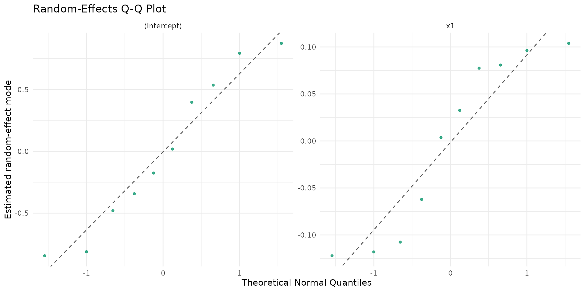
7) Random-effects study (numeric + visual)

rs <- brsmm_re_study(fit_rs)
print(rs)
#> 
#> Random-effects study
#> Groups: 10 
#> 
#> Random-effects (VarCorr):
#>   Name                      Std.Dev.  Corr
#>   (Intercept)                 0.3240
#>   x1                          0.2200  0.9992
#> 
#> ICC (logit(Y) scale, beta level-1 variance): 0.0804
#> 
#> Summary by term (SD_model = model SD; shrinkage = Var(modes)/Var(model)):
#>         term sd_model mean_mode sd_mode shrinkage_ratio shapiro_p
#>  (Intercept)    0.324   -0.0044  0.2795          0.7441    0.1585
#>           x1    0.220   -0.0030  0.1897          0.7436    0.1585
kbl10(rs$summary)

term	sd_model	mean_mode	sd_mode	shrinkage_ratio	shapiro_p
(Intercept)	0.324	-0.0044	0.2795	0.7441	0.1585
x1	0.220	-0.0030	0.1897	0.7436	0.1585

kbl10(rs$D)

	(Intercept)	x1
(Intercept)	0.1050	0.0712
x1	0.0712	0.0484

kbl10(rs$Corr)

	(Intercept)	x1
(Intercept)	1.0000	0.9992
x1	0.9992	1.0000

if (requireNamespace("ggplot2", quietly = TRUE)) {
  autoplot.brsmm(fit_rs, type = "ranef_caterpillar")
  autoplot.brsmm(fit_rs, type = "ranef_density")
  autoplot.brsmm(fit_rs, type = "ranef_pairs")
  autoplot.brsmm(fit_rs, type = "ranef_qq")
}

8) A Monte Carlo study (design of Lopes, 2023, ch. 3)

A simulation study is a loop of brs_sim() and brs() over a fixed design. The code below mirrors the dissertation’s design with a smaller grid: repar 2 with logit links, interval = "mid", two scale lengths ( $K=10$ and $K=100$ ), two sample sizes and three dispersion levels, 200 replicates per cell. It takes under a minute, so it is not run here.

R <- 200L
beta <- c(0.5, 0.2, -0.7)
grid <- expand.grid(sigma = c(0.08, 0.2, 0.4), n = c(100L, 500L), K = c(10L, 100L))
one_cell <- function(sigma, n, K) {
  set.seed(1000 + n + K + round(100 * sigma))
  d <- data.frame(x1 = rnorm(n), x2 = rbinom(n, 1, 0.5))   # fixed design
  truth <- c(beta, qlogis(sigma))
  est <- se <- matrix(NA_real_, R, 4)
  for (r in seq_len(R)) {
    s <- brs_sim(~ x1 + x2, data = d, beta = beta, phi = qlogis(sigma), ncuts = K)
    f <- tryCatch(brs(y ~ x1 + x2, data = s), error = function(e) NULL)
    if (is.null(f) || f$convergence != 0L) next
    est[r, ] <- coef(f)
    se[r, ] <- sqrt(diag(vcov(f)))
  }
  ok <- stats::complete.cases(est, se)
  err <- est[ok, ] - rep(truth, each = sum(ok))
  data.frame(sigma, n, K, par = c("b0", "b1", "b2", "logit_sigma"),
             bias = colMeans(err), rmse = sqrt(colMeans(err^2)),
             cover = colMeans(abs(err) <= qnorm(0.975) * se[ok, ]))
}
res <- do.call(rbind, Map(one_cell, grid$sigma, grid$n, grid$K))

Results for the slope $\beta_1=0.2$ and for $\mathrm{logit}(\sigma)$ (bias, root mean squared error and coverage of the 95% Wald interval, with the default compiled Hessian; hessian_method = "numDeriv" gives the same coverages):

$K$	$n$	$\sigma$	$\beta_1$ bias	RMSE	cover	$\mathrm{logit}\,\sigma$ bias	RMSE	cover
10	100	0.08	0.003	0.057	0.925	-0.047	0.160	0.920
10	100	0.20	0.009	0.092	0.925	-0.038	0.146	0.945
10	100	0.40	-0.011	0.127	0.945	-0.024	0.141	0.945
10	500	0.08	0.000	0.029	0.920	-0.013	0.067	0.930
10	500	0.20	0.005	0.039	0.975	-0.004	0.061	0.945
10	500	0.40	-0.003	0.060	0.945	-0.013	0.059	0.945
100	100	0.08	-0.003	0.055	0.955	-0.047	0.132	0.965
100	100	0.20	0.006	0.097	0.930	-0.043	0.138	0.935
100	100	0.40	0.014	0.113	0.940	-0.046	0.131	0.935
100	500	0.08	0.002	0.031	0.920	-0.012	0.064	0.930
100	500	0.20	0.001	0.040	0.945	-0.003	0.059	0.955
100	500	0.40	0.008	0.063	0.930	-0.004	0.057	0.940

With 200 replicates the Monte Carlo standard error of a coverage near 0.95 is about 0.015. The slopes are unbiased at both scale lengths; the dispersion is slightly underestimated at $n=100$ (about $-0.04$ on the logit scale, a third of its RMSE) and the bias vanishes at $n=500$ . A coarse scale ( $K=10$ ) costs little precision relative to $K=100$ .

9) Practical decision checklist

Start with brs candidates (link, repar) and rank them using brs_table().
Add bootstrap analysis and Average Marginal Effects (AME) before escalating complexity.
Use brs_cv() for out-of-sample stability checks.
Escalate to brsmm only when LR/AIC/BIC metrics and diagnostics clearly support it.
For random slopes, always inspect brsmm_re_study() and the associated random-effects plots.
Read the one-line warnings of brs()/brsmm() (gradient, Hessian, clamps, variance at the boundary) before any Wald statement; fit$diagnostics keeps the numbers.

References

Lopes, J. E. (2023). Modelos de regressão beta para dados de escala. Master’s dissertation, Universidade Federal do Paraná, Curitiba. https://hdl.handle.net/1884/86624.

Self, S. G., and Liang, K.-Y. (1987). Asymptotic properties of maximum likelihood estimators and likelihood ratio tests under nonstandard conditions. Journal of the American Statistical Association, 82(398), 605-610.

Stram, D. O., and Lee, J. W. (1994). Variance components testing in the longitudinal mixed effects model. Biometrics, 50(4), 1171-1177.

Ferrari, S. L. P. and Cribari-Neto, F. (2004). Beta regression for modelling rates and proportions. Journal of Applied Statistics, 31(7), 799-815. DOI: 10.1080/0266476042000214501. Validated online via: https://doi.org/10.1080/0266476042000214501.

Smithson, M., and Verkuilen, J. (2006). A better lemon squeezer? Maximum-likelihood regression with beta-distributed dependent variables. Psychological Methods, 11(1), 54-71. DOI: 10.1037/1082-989X.11.1.54. Validated online via: https://doi.org/10.1037/1082-989X.11.1.54.

Rue, H., Martino, S., and Chopin, N. (2009). Approximate Bayesian inference for latent Gaussian models by using integrated nested Laplace approximations. Journal of the Royal Statistical Society: Series B, 71(2), 319-392. DOI: 10.1111/j.1467-9868.2008.00700.x. Validated online via: https://doi.org/10.1111/j.1467-9868.2008.00700.x.