Overview
brsmm() extends brs() to clustered data by
adding Gaussian random effects in the mean submodel while preserving the
interval-censored beta likelihood for scale-derived outcomes.
This vignette covers:
- full model mathematics;
- estimation by marginal maximum likelihood (Laplace approximation);
- practical use of all current
brsmmmethods; - inferential and validation workflows, including parameter recovery.
Mathematical model
Assume observations within groups , with group-specific random-effects vector .
Linear predictors
with
and
chosen by link and link_phi. The
random-effects design row
is defined by random = ~ terms | group.
Beta parameterization
For each
,
repar maps to beta shape parameters
via brs_repar().
Conditional contribution by censoring type
Each observation contributes:
where are interval endpoints on , is beta density, and is beta CDF.
Random-effects distribution
where
is a symmetric positive-definite covariance matrix. Internally,
brsmm() optimizes a packed lower-Cholesky parameterization
(diagonal entries on log-scale for positivity).
Laplace approximation used by brsmm()
Define and , with curvature Then
brsmm() maximizes the approximated
with stats::optim(), and computes group-level posterior
modes
.
For
,
this reduces to the scalar random-intercept formula.
Simulating clustered scale data
The next helper simulates data from a known mixed model to illustrate fitting, inference, and recovery checks.
sim_brsmm_data <- function(seed = 3501L, g = 24L, ni = 12L,
                           beta = c(0.20, 0.65),
                           gamma = c(-0.15),
                           sigma_b = 0.55) {
  set.seed(seed)
  id <- factor(rep(seq_len(g), each = ni))
  n <- length(id)
  x1 <- rnorm(n)

  b_true <- rnorm(g, mean = 0, sd = sigma_b)
  eta_mu <- beta[1] + beta[2] * x1 + b_true[as.integer(id)]
  eta_phi <- rep(gamma[1], n)

  mu <- plogis(eta_mu)
  phi <- plogis(eta_phi)
  shp <- brs_repar(mu = mu, phi = phi, repar = 2)
  y <- round(stats::rbeta(n, shp$shape1, shp$shape2) * 100)

  list(
    data = data.frame(y = y, x1 = x1, id = id),
    truth = list(beta = beta, gamma = gamma, sigma_b = sigma_b, b = b_true)
  )
}

sim <- sim_brsmm_data(
  g = 5,
  ni = 200,
  beta = c(0.20, 0.65),
  gamma = c(-0.15),
  sigma_b = 0.55
)
str(sim$data)
#> 'data.frame':    1000 obs. of  3 variables:
#>  $ y : num  92 0 71 59 21 5 34 1 19 0 ...
#>  $ x1: num  -0.3677 -2.0069 -0.0469 -0.2468 0.7634 ...
#>  $ id: Factor w/ 5 levels "1","2","3","4",..: 1 1 1 1 1 1 1 1 1 1 ...
Fitting brsmm()
fit_mm <- brsmm(
  y ~ x1,
  random = ~ 1 | id,
  data = sim$data,
  repar = 2,
  int_method = "laplace",
  method = "BFGS",
  control = list(maxit = 1000)
)

summary(fit_mm)
#>
#> Call:
#> brsmm(formula = y ~ x1, random = ~1 | id, data = sim$data, repar = 2,
#>     int_method = "laplace", method = "BFGS", control = list(maxit = 1000))
#>
#> Randomized Quantile Residuals:
#>     Min      1Q  Median      3Q     Max
#> -2.8356 -0.6727 -0.0422  0.6041  3.0834
#>
#> Coefficients (mean model with logit link):
#>             Estimate Std. Error z value Pr(>|z|)
#> (Intercept)  0.26228    0.18100   1.449    0.147
#> x1           0.63847    0.04381  14.572   <2e-16 ***
#> ---
#> Signif. codes:  0 '***' 0.001 '**' 0.01 '*' 0.05 '.' 0.1 ' ' 1
#>
#> Phi coefficients (precision model with logit link):
#>             Estimate Std. Error z value Pr(>|z|)
#> (Intercept) -0.10608    0.04044  -2.623  0.00871 **
#> ---
#> Signif. codes:  0 '***' 0.001 '**' 0.01 '*' 0.05 '.' 0.1 ' ' 1
#>
#> Random-effects parameters (Cholesky scale):
#>                      Estimate Std. Error z value Pr(>|z|)
#> logSD.(Intercept)|id  -0.9284     0.3339   -2.78  0.00543 **
#> ---
#> Signif. codes:  0 '***' 0.001 '**' 0.01 '*' 0.05 '.' 0.1 ' ' 1
#> ---
#> Mixed beta interval model (Laplace)
#> Observations: 1000  | Groups: 5
#> Log-likelihood: -4182.1094 on 4 Df | AIC: 8372.2188 | BIC: 8391.8498
#> Pseudo R-squared: 0.1815
#> Number of iterations: 27 (BFGS)
#> Censoring: 852 interval | 39 left | 109 right
Random intercept + slope example
The model below includes a random intercept and random slope for
x1:
fit_mm_rs <- brsmm(
  y ~ x1,
  random = ~ 1 + x1 | id,
  data = sim$data,
  repar = 2,
  int_method = "laplace",
  method = "BFGS",
  control = list(maxit = 1200)
)

summary(fit_mm_rs)
#>
#> Call:
#> brsmm(formula = y ~ x1, random = ~1 + x1 | id, data = sim$data,
#>     repar = 2, int_method = "laplace", method = "BFGS", control = list(maxit = 1200))
#>
#> Randomized Quantile Residuals:
#>     Min      1Q  Median      3Q     Max
#> -3.6103 -0.6735 -0.0460  0.6225  3.9921
#>
#> Coefficients (mean model with logit link):
#>             Estimate Std. Error z value Pr(>|z|)
#> (Intercept)  0.25933    0.18132    1.43    0.153
#> x1           0.63732    0.04571   13.94   <2e-16 ***
#> ---
#> Signif. codes:  0 '***' 0.001 '**' 0.01 '*' 0.05 '.' 0.1 ' ' 1
#>
#> Phi coefficients (precision model with logit link):
#>             Estimate Std. Error z value Pr(>|z|)
#> (Intercept) -0.10618    0.04053   -2.62   0.0088 **
#> ---
#> Signif. codes:  0 '***' 0.001 '**' 0.01 '*' 0.05 '.' 0.1 ' ' 1
#>
#> Random-effects parameters (Cholesky scale):
#>                       Estimate Std. Error z value Pr(>|z|)
#> logSD.(Intercept)|id  -0.92450    0.33463  -2.763  0.00573 **
#> cov.x1:(Intercept)|id -0.02748    0.04491  -0.612  0.54064
#> logSD.x1|id           -4.65173    4.06768  -1.144  0.25280
#> ---
#> Signif. codes:  0 '***' 0.001 '**' 0.01 '*' 0.05 '.' 0.1 ' ' 1
#> ---
#> Mixed beta interval model (Laplace)
#> Observations: 1000  | Groups: 5
#> Log-likelihood: -4181.9349 on 6 Df | AIC: 8375.8699 | BIC: 8405.3164
#> Pseudo R-squared: 0.1815
#> Number of iterations: 69 (BFGS)
#> Censoring: 852 interval | 39 left | 109 right
Covariance structure of random effects:
kbl10(fit_mm_rs$random$D)| V1 | V2 |
|---|---|
| 0.1574 | -0.0109 |
| -0.0109 | 0.0008 |
kbl10(
  data.frame(term = names(fit_mm_rs$random$sd_b), sd = as.numeric(fit_mm_rs$random$sd_b)),
  digits = 4
)| term | sd |
|---|---|
| (Intercept) | 0.3967 |
| x1 | 0.0291 |
| (Intercept) | x1 |
|---|---|
| -0.5181 | 0.0357 |
| 0.6224 | -0.0432 |
| -0.2464 | 0.0170 |
| 0.1490 | -0.0111 |
| 0.0050 | 0.0007 |
Additional studies of random effects (numerical and visual)
Following practices from established mixed-models packages, the package now allows for a dedicated study of the random effects focusing on:
- structure and correlation;
- empirical distribution of modes by group;
- empirical shrinkage intensity;
- specific visual diagnostics for the random components.
re_study <- brsmm_re_study(fit_mm_rs)
print(re_study)
#>
#> Random-effects study
#> Groups: 5
#>
#> Random-effects (VarCorr):
#>   Name                      Std.Dev.  Corr
#>   re1                         0.3967
#>   re2                         0.0291  -0.9446
#>
#> ICC (latent logistic scale): 0.0457
#>
#> Summary by term (SD_model = model SD; shrinkage = Var(modes)/Var(model)):
#>         term sd_model mean_mode sd_mode shrinkage_ratio shapiro_p
#>  (Intercept)   0.3967    0.0024  0.4297               1    0.9640
#>           x1   0.0291   -0.0002  0.0298               1    0.9687
kbl10(re_study$summary)| term | sd_model | mean_mode | sd_mode | shrinkage_ratio | shapiro_p |
|---|---|---|---|---|---|
| (Intercept) | 0.3967 | 0.0024 | 0.4297 | 1 | 0.9640 |
| x1 | 0.0291 | -0.0002 | 0.0298 | 1 | 0.9687 |
kbl10(re_study$D)| V1 | V2 |
|---|---|
| 0.1574 | -0.0109 |
| -0.0109 | 0.0008 |
kbl10(re_study$Corr)| V1 | V2 |
|---|---|
| 1.0000 | -0.9446 |
| -0.9446 | 1.0000 |
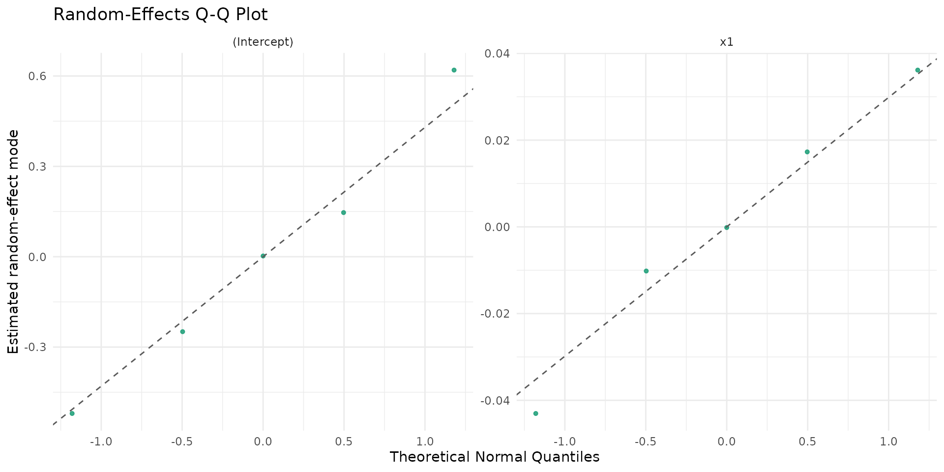
Suggested visualizations for random effects:
if (requireNamespace("ggplot2", quietly = TRUE)) {
  autoplot.brsmm(fit_mm_rs, type = "ranef_caterpillar")
  autoplot.brsmm(fit_mm_rs, type = "ranef_density")
  autoplot.brsmm(fit_mm_rs, type = "ranef_pairs")
  autoplot.brsmm(fit_mm_rs, type = "ranef_qq")
}
Core methods
Coefficients and random effects
coef(fit_mm, model = "random") returns packed
random-effect covariance parameters on the optimizer scale
(lower-Cholesky, with a log-diagonal). For random-intercept models, this
simplifies to
.
kbl10(
  data.frame(
    parameter = names(coef(fit_mm, model = "full")),
    estimate = as.numeric(coef(fit_mm, model = "full"))
  ),
  digits = 4
)| parameter | estimate |
|---|---|
| (Intercept) | 0.2623 |
| x1 | 0.6385 |
| (phi)_(Intercept) | -0.1061 |
| (re_chol_logsd)_(Intercept)|id | -0.9284 |
kbl10(
  data.frame(
    log_sigma_b = as.numeric(coef(fit_mm, model = "random")),
    sigma_b = as.numeric(exp(coef(fit_mm, model = "random")))
  ),
  digits = 4
)| log_sigma_b | sigma_b |
|---|---|
| -0.9284 | 0.3952 |
| x |
|---|
| -0.5219 |
| 0.6188 |
| -0.2498 |
| 0.1421 |
| 0.0084 |
For random intercept + slope models:
kbl10(
  data.frame(
    parameter = names(coef(fit_mm_rs, model = "random")),
    estimate = as.numeric(coef(fit_mm_rs, model = "random"))
  ),
  digits = 4
)| parameter | estimate |
|---|---|
| (re_chol_logsd)_(Intercept)|id | -0.9245 |
| (re_chol)_x1:(Intercept)|id | -0.0275 |
| (re_chol_logsd)_x1|id | -4.6517 |
kbl10(fit_mm_rs$random$D)| V1 | V2 |
|---|---|
| 0.1574 | -0.0109 |
| -0.0109 | 0.0008 |
Variance-covariance, summary and likelihood criteria
| mean.Estimate | mean.Std..Error | mean.z.value | mean.Pr…z.. | precision.Estimate | precision.Std..Error | precision.z.value | precision.Pr…z.. | random.Estimate | random.Std..Error | random.z.value | random.Pr…z.. | |
|---|---|---|---|---|---|---|---|---|---|---|---|---|
| (Intercept) | 0.2623 | 0.1810 | 1.4490 | 0.1473 | -0.1061 | 0.0404 | -2.6231 | 0.0087 | -0.9284 | 0.3339 | -2.7802 | 0.0054 |
| x1 | 0.6385 | 0.0438 | 14.5724 | 0.0000 | -0.1061 | 0.0404 | -2.6231 | 0.0087 | -0.9284 | 0.3339 | -2.7802 | 0.0054 |
kbl10(
  data.frame(
    logLik = as.numeric(logLik(fit_mm)),
    AIC = AIC(fit_mm),
    BIC = BIC(fit_mm),
    nobs = nobs(fit_mm)
  ),
  digits = 4
)| logLik | AIC | BIC | nobs |
|---|---|---|---|
| -4182.109 | 8372.219 | 8391.85 | 1000 |
Fitted values, prediction and residuals
kbl10(
  data.frame(
    mu_hat = head(fitted(fit_mm, type = "mu")),
    phi_hat = head(fitted(fit_mm, type = "phi")),
    pred_mu = head(predict(fit_mm, type = "response")),
    pred_eta = head(predict(fit_mm, type = "link")),
    pred_phi = head(predict(fit_mm, type = "precision")),
    pred_var = head(predict(fit_mm, type = "variance"))
  ),
  digits = 4
)| mu_hat | phi_hat | pred_mu | pred_eta | pred_phi | pred_var |
|---|---|---|---|---|---|
| 0.3789 | 0.4735 | 0.3789 | -0.4944 | 0.4735 | 0.1114 |
| 0.1764 | 0.4735 | 0.1764 | -1.5410 | 0.4735 | 0.0688 |
| 0.4281 | 0.4735 | 0.4281 | -0.2896 | 0.4735 | 0.1159 |
| 0.3972 | 0.4735 | 0.3972 | -0.4172 | 0.4735 | 0.1134 |
| 0.5567 | 0.4735 | 0.5567 | 0.2278 | 0.4735 | 0.1169 |
| 0.3379 | 0.4735 | 0.3379 | -0.6729 | 0.4735 | 0.1059 |
kbl10(
  data.frame(
    res_response = head(residuals(fit_mm, type = "response")),
    res_pearson = head(residuals(fit_mm, type = "pearson"))
  ),
  digits = 4
)| res_response | res_pearson |
|---|---|
| 0.5411 | 1.6211 |
| -0.1764 | -0.6725 |
| 0.2819 | 0.8279 |
| 0.1928 | 0.5727 |
| -0.3467 | -1.0142 |
| -0.2879 | -0.8844 |
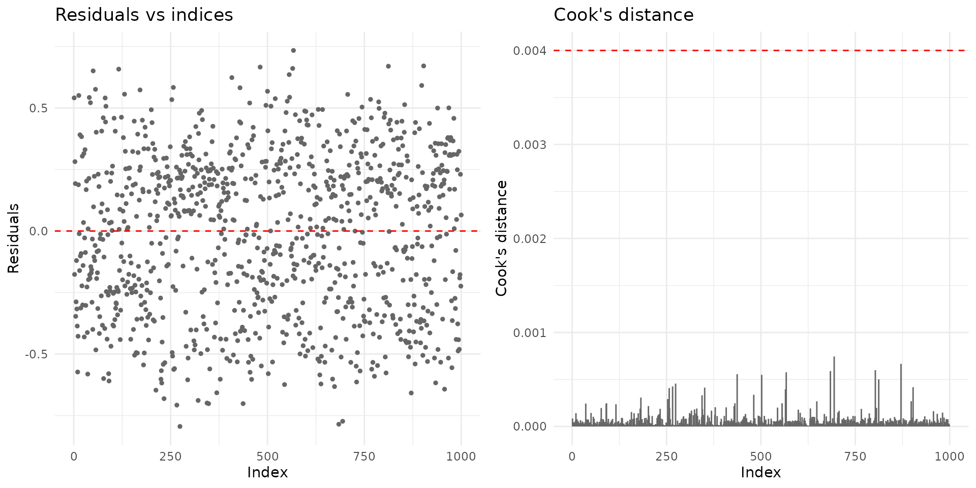
Diagnostic plotting methods
plot.brsmm() supports base and ggplot2 backends:
plot(fit_mm, which = 1:4, type = "pearson")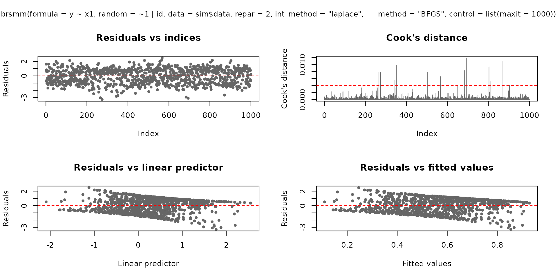
if (requireNamespace("ggplot2", quietly = TRUE)) {
  plot(fit_mm, which = 1:2, gg = TRUE)
}
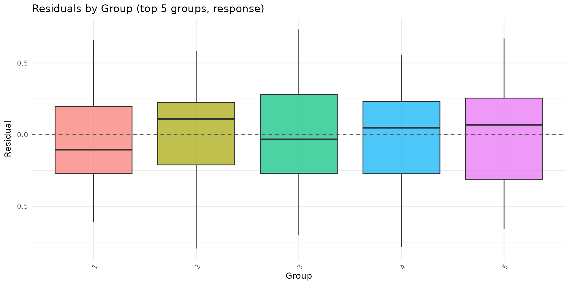
autoplot.brsmm() provides focused ggplot
diagnostics:
if (requireNamespace("ggplot2", quietly = TRUE)) {
  autoplot.brsmm(fit_mm, type = "calibration")
  autoplot.brsmm(fit_mm, type = "score_dist")
  autoplot.brsmm(fit_mm, type = "ranef_qq")
  autoplot.brsmm(fit_mm, type = "residuals_by_group")
}
Prediction with newdata
If newdata contains unseen groups,
predict.brsmm() uses a random effect equal to zero for
those levels.
nd <- sim$data[1:8, c("x1", "id")]
kbl10(
  data.frame(pred_seen = as.numeric(predict(fit_mm, newdata = nd, type = "response"))),
  digits = 4
)| pred_seen |
|---|
| 0.3789 |
| 0.1764 |
| 0.4281 |
| 0.3972 |
| 0.5567 |
| 0.3379 |
| 0.4600 |
| 0.3268 |
nd_unseen <- nd
nd_unseen$id <- factor(rep("new_cluster", nrow(nd_unseen)))
kbl10(
  data.frame(pred_unseen = as.numeric(predict(fit_mm, newdata = nd_unseen, type = "response"))),
  digits = 4
)| pred_unseen |
|---|
| 0.5069 |
| 0.2652 |
| 0.5578 |
| 0.5262 |
| 0.6791 |
| 0.4623 |
| 0.5895 |
| 0.4499 |
The same logic applies to random intercept + slope models:
kbl10(
  data.frame(pred_rs_seen = as.numeric(predict(fit_mm_rs, newdata = nd, type = "response"))),
  digits = 4
)| pred_rs_seen |
|---|
| 0.3761 |
| 0.1667 |
| 0.4279 |
| 0.3954 |
| 0.5634 |
| 0.3331 |
| 0.4616 |
| 0.3215 |
kbl10(
  data.frame(pred_rs_unseen = as.numeric(predict(fit_mm_rs, newdata = nd_unseen, type = "response"))),
  digits = 4
)| pred_rs_unseen |
|---|
| 0.5062 |
| 0.2651 |
| 0.5571 |
| 0.5255 |
| 0.6783 |
| 0.4618 |
| 0.5887 |
| 0.4494 |
Statistical tests and validation workflow
Wald tests (from summary)
summary.brsmm() reports Wald
-tests
for each parameter:
sm <- summary(fit_mm)
kbl10(sm$coefficients)| mean.Estimate | mean.Std..Error | mean.z.value | mean.Pr…z.. | precision.Estimate | precision.Std..Error | precision.z.value | precision.Pr…z.. | random.Estimate | random.Std..Error | random.z.value | random.Pr…z.. | |
|---|---|---|---|---|---|---|---|---|---|---|---|---|
| (Intercept) | 0.2623 | 0.1810 | 1.4490 | 0.1473 | -0.1061 | 0.0404 | -2.6231 | 0.0087 | -0.9284 | 0.3339 | -2.7802 | 0.0054 |
| x1 | 0.6385 | 0.0438 | 14.5724 | 0.0000 | -0.1061 | 0.0404 | -2.6231 | 0.0087 | -0.9284 | 0.3339 | -2.7802 | 0.0054 |
Evolutionary scheme and Likelihood Ratio (LR) test selection
A practical workflow of increasing complexity:
-
brs(): no random effect (ignores clustering); -
brsmm(..., random = ~ 1 | id): random intercept; -
brsmm(..., random = ~ 1 + x1 | id): random intercept + slope.
In the first jump (brs to brsmm with
intercept), the hypothesis
lies on the boundary of the parameter space. Thus, the classical
asymptotic
reference distribution should be interpreted with caution. In the second
jump (intercept to intercept + slope), the Likelihood Ratio (LR) test
with a
distribution is commonly used as a practical diagnostic for
goodness-of-fit gains.
# Base model without a random effect
fit_brs <- brs(
  y ~ x1,
  data = sim$data,
  repar = 2
)

# Reuse the mixed models already fitted:
# fit_mm    : random = ~ 1 | id
# fit_mm_rs : random = ~ 1 + x1 | id

tab_lr <- anova(fit_brs, fit_mm, fit_mm_rs, test = "Chisq")
kbl10(
  data.frame(model = rownames(tab_lr), tab_lr, row.names = NULL),
  digits = 4
)| model | Df | logLik | AIC | BIC | Chisq | Chi.Df | Pr..Chisq. |
|---|---|---|---|---|---|---|---|
| M1 (brs) | 3 | -4219.025 | 8444.051 | 8458.774 | NA | NA | NA |
| M2 (brsmm) | 4 | -4182.109 | 8372.219 | 8391.850 | 73.8319 | 1 | 0.0000 |
| M3 (brsmm) | 6 | -4181.935 | 8375.870 | 8405.316 | 0.3489 | 2 | 0.8399 |
Operational decision rule (analytical):
- If the second jump (RI to RI+RS) does not improve the fit (high p-value), prefer the random-intercept model for parsimony.
- If there is a robust gain, adopt the RI+RS model and validate
parameter stability (especially
sd_band the matrix) via sensitivity and residual diagnostics.
Residual diagnostics (quick checks)
r <- residuals(fit_mm, type = "pearson")
kbl10(
  data.frame(
    mean = mean(r),
    sd = stats::sd(r),
    q025 = as.numeric(stats::quantile(r, 0.025)),
    q975 = as.numeric(stats::quantile(r, 0.975))
  ),
  digits = 4
)| mean | sd | q025 | q975 |
|---|---|---|---|
| -0.0328 | 0.9963 | -1.8841 | 1.5617 |
Parameter recovery experiment
A single-fit recovery table can be produced directly from the previous fit:
est <- c(
  beta0 = unname(coef(fit_mm, model = "mean")[1]),
  beta1 = unname(coef(fit_mm, model = "mean")[2]),
  sigma_b = unname(exp(coef(fit_mm, model = "random")))
)

true <- c(
  beta0 = sim$truth$beta[1],
  beta1 = sim$truth$beta[2],
  sigma_b = sim$truth$sigma_b
)

recovery_table <- data.frame(
  parameter = names(true),
  true = as.numeric(true),
  estimate = as.numeric(est[names(true)]),
  bias = as.numeric(est[names(true)] - true)
)
kbl10(recovery_table)| parameter | true | estimate | bias |
|---|---|---|---|
| beta0 | 0.20 | 0.2623 | 0.0623 |
| beta1 | 0.65 | 0.6385 | -0.0115 |
| sigma_b | 0.55 | 0.3952 | -0.1548 |
For a Monte Carlo recovery study, repeat simulation and fitting across replicates:
mc_recovery <- function(R = 50L, seed = 7001L) {
  set.seed(seed)
  out <- vector("list", R)

  for (r in seq_len(R)) {
    sim_r <- sim_brsmm_data(seed = seed + r)
    fit_r <- brsmm(
      y ~ x1,
      random = ~ 1 | id,
      data = sim_r$data,
      repar = 2,
      int_method = "laplace",
      method = "BFGS",
      control = list(maxit = 1000)
    )

    out[[r]] <- c(
      beta0 = unname(coef(fit_r, model = "mean")[1]),
      beta1 = unname(coef(fit_r, model = "mean")[2]),
      sigma_b = unname(exp(coef(fit_r, model = "random")))
    )
  }

  est <- do.call(rbind, out)
  truth <- c(beta0 = 0.20, beta1 = 0.65, sigma_b = 0.55)

  data.frame(
    parameter = colnames(est),
    truth = as.numeric(truth[colnames(est)]),
    mean_est = colMeans(est),
    bias = colMeans(est) - truth[colnames(est)],
    rmse = sqrt(colMeans((sweep(est, 2, truth[colnames(est)], "-"))^2))
  )
}

kbl10(mc_recovery(R = 50))
How this maps to automated package tests
The package test suite includes dedicated brsmm tests
for:
- fitting with Laplace integration;
- one- and two-part formulas;
- S3 methods (
coef,vcov,summary,predict,residuals,ranef); - parameter recovery under known DGP settings.
Run locally:
devtools::test(filter = "brsmm")References
Ferrari, S. L. P. and Cribari-Neto, F. (2004). Beta regression for modelling rates and proportions. Journal of Applied Statistics, 31(7), 799-815. DOI: 10.1080/0266476042000214501. Validated online via: https://doi.org/10.1080/0266476042000214501.
Pinheiro, J. C. and Bates, D. M. (2000). Mixed-Effects Models in S and S-PLUS. Springer. DOI: 10.1007/b98882. Validated online via: https://doi.org/10.1007/b98882.
Rue, H., Martino, S., and Chopin, N. (2009). Approximate Bayesian inference for latent Gaussian models by using integrated nested Laplace approximations. Journal of the Royal Statistical Society: Series B, 71(2), 319-392. DOI: 10.1111/j.1467-9868.2008.00700.x. Validated online via: https://doi.org/10.1111/j.1467-9868.2008.00700.x.