Introduction to betaregscale

Overview

The betaregscale package provides maximum-likelihood estimation of beta regression models for responses derived from bounded rating scales. Common examples include pain intensity scales (NRS-11, NRS-21, NRS-101), Likert-type scales, product quality ratings, and any instrument whose response can be mapped to the open interval $(0,1)$.

The key idea is that a discrete score recorded on a bounded scale carries measurement uncertainty inherent to the instrument. For instance, a pain score of $y=6$ on a 0–10 NRS is not an exact value but rather represents a range: after rescaling to $(0,1)$, the observation is treated as interval-censored in $[0.55,0.65]$. The package uses the beta distribution to model such data, building a complete likelihood that supports mixed censoring types within the same dataset.

Installation

# Development version from GitHub:
# install.packages("remotes")
remotes::install_github("evandeilton/betaregscale")

library(betaregscale)

Censoring types

The complete likelihood supports four censoring types, automatically classified by brs_check():

$\delta$	Type	Likelihood contribution
0	Exact (uncensored)	$f(y_i;a_i,b_i)$
1	Left-censored ($y=0$)	$F(u_i;a_i,b_i)$
2	Right-censored ($y=K$)	$1-F(l_i;a_i,b_i)$
3	Interval-censored	$F(u_i;a_i,b_i)-F(l_i;a_i,b_i)$

where $f(\cdot)$ and $F(\cdot)$ are the beta density and CDF, $[l_i,u_i]$ are the interval endpoints, and $(a_i,b_i)$ are the beta shape parameters derived from $\mu_i$ and $\phi_i$ via the chosen reparameterization.

Interval construction

Scale observations are mapped to $(0,1)$ with midpoint uncertainty intervals:

$$y_t=y/K,\quad\text{interval }[y_t-h/K,y_t+h/K]$$

where $K$ is the number of scale categories (ncuts) and $h$ is the half-width (lim, default 0.5).

# Illustrate brs_check with a 0-10 NRS scale
y_example <- c(0, 3, 5, 7, 10)
cr <- brs_check(y_example, ncuts = 10)
kbl10(cr)

left	right	yt	y	delta
0.00	0.05	0.0	0	1
0.25	0.35	0.3	3	3
0.45	0.55	0.5	5	3
0.65	0.75	0.7	7	3
0.95	1.00	1.0	10	2

The delta column shows that $y=0$ is left-censored ($\delta=1$), $y=10$ is right-censored ($\delta=2$), and all interior values are interval-censored ($\delta=3$).

Data preparation with brs_prep()

In practice, analysts may want to supply their own censoring indicators or interval endpoints rather than relying on the automatic classification of brs_check(). The brs_prep() function provides a flexible, validated bridge between raw analyst data and brs().

It supports four input modes:

Mode 1: Score only (automatic)

# Equivalent to brs_check - delta inferred from y
d1 <- data.frame(y = c(0, 3, 5, 7, 10), x1 = rnorm(5))
kbl10(brs_prep(d1, ncuts = 10))

left	right	yt	y	delta	x1
0.00	0.05	0.0	0	1	-1.4000
0.25	0.35	0.3	3	3	0.2553
0.45	0.55	0.5	5	3	-2.4373
0.65	0.75	0.7	7	3	-0.0056
0.95	1.00	1.0	10	2	0.6216

Mode 2: Score + explicit censoring indicator

# Analyst specifies delta directly
d2 <- data.frame(
  y     = c(50, 0, 99, 50),
  delta = c(0, 1, 2, 3),
  x1    = rnorm(4)
)
kbl10(brs_prep(d2, ncuts = 100))

left	right	yt	y	delta	x1
0.500	0.500	0.50	50	0	1.1484
0.000	0.005	0.00	0	1	-1.8218
0.985	1.000	0.99	99	2	-0.2473
0.495	0.505	0.50	50	3	-0.2442

Mode 3: Interval endpoints with NA patterns

When the analyst provides left and/or right columns, censoring is inferred from the NA pattern:

d3 <- data.frame(
  left  = c(NA, 20, 30, NA),
  right = c(5, NA, 45, NA),
  y     = c(NA, NA, NA, 50),
  x1    = rnorm(4)
)
kbl10(brs_prep(d3, ncuts = 100))

left	right	yt	y	delta	x1
0.0	0.05	0.025	NA	1	-0.2827
0.2	1.00	0.600	NA	2	-0.5537
0.3	0.45	0.375	NA	3	0.6290
0.5	0.50	0.500	50	0	2.0650

Mode 4: Analyst-supplied intervals

When the analyst provides y, left, and right simultaneously, their endpoints are used directly (rescaled by $K$):

d4 <- data.frame(
  y     = c(50, 75),
  left  = c(48, 73),
  right = c(52, 77),
  x1    = rnorm(2)
)
kbl10(brs_prep(d4, ncuts = 100))

left	right	yt	y	delta	x1
0.48	0.52	0.50	50	3	-1.6310
0.73	0.77	0.75	75	3	0.5124

Using brs_prep with brs()

Data processed by brs_prep() is automatically detected by brs() - the internal brs_check() step is skipped:

set.seed(42)
n <- 1000
dat <- data.frame(x1 = rnorm(n), x2 = rnorm(n))
sim <- brs_sim(
  formula = ~ x1 + x2, data = dat,
  beta = c(0.2, -0.5, 0.3), phi = 0.3,
  link = "logit", link_phi = "logit",
  repar = 2
)
# Remove left, right, yt so brs_prep can rebuild them
prep <- brs_prep(sim[-c(1:3)], ncuts = 100)
fit_prep <- brs(y ~ x1 + x2,
  data = prep, repar = 2,
  link = "logit", link_phi = "logit"
)
summary(fit_prep, digits = 4)
#> 
#> Call:
#> brs(formula = y ~ x1 + x2, data = prep, link = "logit", link_phi = "logit", 
#>     repar = 2)
#> 
#> Quantile residuals:
#>     Min      1Q  Median      3Q     Max 
#> -3.1122 -0.6590 -0.0288  0.6409  3.6970 
#> 
#> Coefficients (mean model with logit link):
#>             Estimate Std. Error z value Pr(>|z|)    
#> (Intercept)  0.18254    0.04364   4.183 2.88e-05 ***
#> x1          -0.48490    0.04491 -10.797  < 2e-16 ***
#> x2           0.26206    0.04447   5.893 3.80e-09 ***
#> ---
#> Signif. codes:  0 '***' 0.001 '**' 0.01 '*' 0.05 '.' 0.1 ' ' 1
#> 
#> Phi coefficients (precision model with logit link):
#>       Estimate Std. Error z value Pr(>|z|)    
#> (phi)  0.26989    0.03992    6.76 1.38e-11 ***
#> ---
#> Signif. codes:  0 '***' 0.001 '**' 0.01 '*' 0.05 '.' 0.1 ' ' 1
#> ---
#> Log-likelihood: -4072.5673 on 4 Df | AIC: 8153.1346 | BIC: 8172.7656 
#> Pseudo R-squared: 0.1292 
#> Number of iterations: 35 (BFGS) 
#> Censoring: 796 interval | 74 left | 130 right

Example 1: Fixed dispersion model

Simulating data

We simulate observations from a beta regression model with fixed dispersion, two covariates, and a logit link for the mean.

set.seed(4255)
n <- 1000
dat <- data.frame(x1 = rnorm(n), x2 = rnorm(n))

sim_fixed <- brs_sim(
  formula  = ~ x1 + x2,
  data     = dat,
  beta     = c(0.3, -0.6, 0.4),
  phi      = 1 / 10,
  link     = "logit",
  link_phi = "logit",
  ncuts    = 100,
  repar    = 2
)

kbl10(head(sim_fixed, 8))

left	right	yt	y	delta	x1	x2
0.165	0.175	0.17	17	3	1.9510	0.2888
0.985	0.995	0.99	99	3	0.7725	1.6103
0.000	0.005	0.00	0	1	0.7264	1.0542
0.575	0.585	0.58	58	3	0.0487	-0.4923
0.095	0.105	0.10	10	3	-0.5445	-1.4098
0.065	0.075	0.07	7	3	0.3600	-1.0116
0.025	0.035	0.03	3	3	0.7136	2.3083
0.355	0.365	0.36	36	3	-0.7274	0.2061

Each observation is centered in its interval. For example, a score of 67 on a 0–100 scale yields $y_t=0.67$ with the interval $[0.665,0.675]$.

Fitting the model

fit_fixed <- brs(
  y ~ x1 + x2,
  data     = sim_fixed,
  link     = "logit",
  link_phi = "logit",
  repar    = 2
)
summary(fit_fixed)
#> 
#> Call:
#> brs(formula = y ~ x1 + x2, data = sim_fixed, link = "logit", 
#>     link_phi = "logit", repar = 2)
#> 
#> Quantile residuals:
#>     Min      1Q  Median      3Q     Max 
#> -3.0753 -0.6600  0.0058  0.7071  3.3708 
#> 
#> Coefficients (mean model with logit link):
#>             Estimate Std. Error z value Pr(>|z|)    
#> (Intercept)  0.30604    0.04312   7.097 1.28e-12 ***
#> x1          -0.60332    0.04530 -13.317  < 2e-16 ***
#> x2           0.44135    0.04385  10.066  < 2e-16 ***
#> ---
#> Signif. codes:  0 '***' 0.001 '**' 0.01 '*' 0.05 '.' 0.1 ' ' 1
#> 
#> Phi coefficients (precision model with logit link):
#>       Estimate Std. Error z value Pr(>|z|)   
#> (phi)  0.10991    0.04057   2.709  0.00674 **
#> ---
#> Signif. codes:  0 '***' 0.001 '**' 0.01 '*' 0.05 '.' 0.1 ' ' 1
#> ---
#> Log-likelihood: -4035.2262 on 4 Df | AIC: 8078.4524 | BIC: 8098.0834 
#> Pseudo R-squared: 0.2393 
#> Number of iterations: 39 (BFGS) 
#> Censoring: 809 interval | 65 left | 126 right

The summary output follows the betareg package style, showing separate coefficient tables for the mean and precision submodels, with Wald z-tests and $p$-values based on the standard normal distribution.

Goodness of fit

kbl10(brs_gof(fit_fixed))

logLik	AIC	BIC	pseudo_r2
-4035.226	8078.452	8098.083	0.2393

Comparing link functions

The package supports several link functions for the mean submodel. We can compare them using information criteria:

links <- c("logit", "probit", "cauchit", "cloglog")
fits <- lapply(setNames(links, links), function(lnk) {
  brs(y ~ x1 + x2, data = sim_fixed, link = lnk, repar = 2)
})

# Estimates
est_table <- do.call(rbind, lapply(names(fits), function(lnk) {
  e <- brs_est(fits[[lnk]])
  e$link <- lnk
  e
}))
kbl10(est_table)

variable	estimate	se	z_value	p_value	ci_lower	ci_upper	link
(Intercept)	0.3060	0.0431	7.0968	0.0000	0.2215	0.3906	logit
x1	-0.6033	0.0453	-13.3169	0.0000	-0.6921	-0.5145	logit
x2	0.4413	0.0438	10.0661	0.0000	0.3554	0.5273	logit
(phi)	0.1099	0.0406	2.7095	0.0067	0.0304	0.1894	logit
(Intercept)	0.1866	0.0262	7.1224	0.0000	0.1352	0.2379	probit
x1	-0.3652	0.0266	-13.7107	0.0000	-0.4175	-0.3130	probit
x2	0.2669	0.0261	10.2177	0.0000	0.2157	0.3181	probit
(phi)	0.1118	0.0405	2.7603	0.0058	0.0324	0.1913	probit
(Intercept)	0.2766	0.0409	6.7671	0.0000	0.1965	0.3566	cauchit
x1	-0.5595	0.0493	-11.3590	0.0000	-0.6561	-0.4630	cauchit

# Goodness of fit
gof_table <- do.call(rbind, lapply(fits, brs_gof))
kbl10(gof_table)

	logLik	AIC	BIC	pseudo_r2
logit	-4035.226	8078.452	8098.083	0.2393
probit	-4035.685	8079.370	8099.001	0.2383
cauchit	-4035.500	8079.000	8098.631	0.1918
cloglog	-4037.563	8083.126	8102.757	0.1824

Residual diagnostics

The plot() method provides six diagnostic panels. By default, the first four are shown:

plot(fit_fixed, caption = NULL, gg = TRUE, title = NULL, theme = ggplot2::theme_bw())

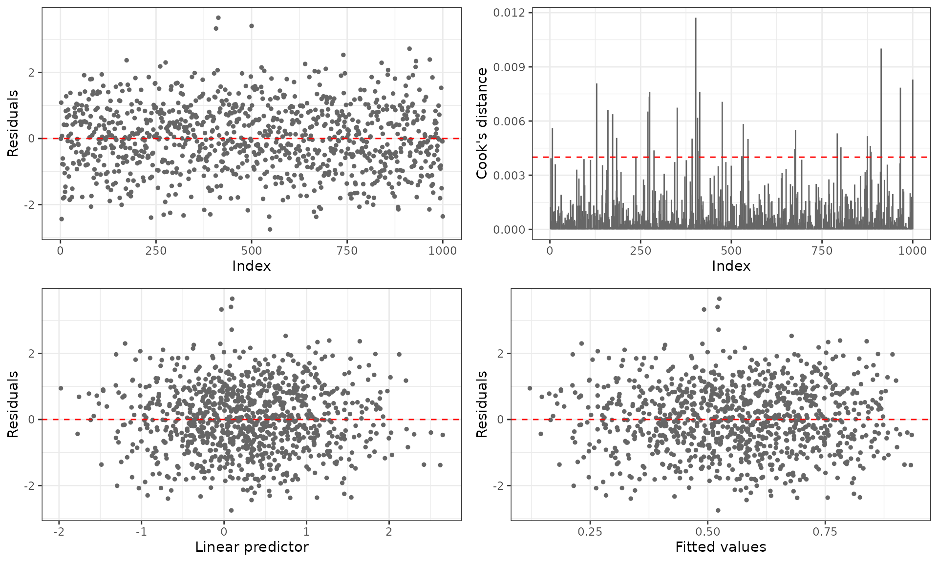
For ggplot2 output (requires the ggplot2 package):

plot(fit_fixed, gg = TRUE)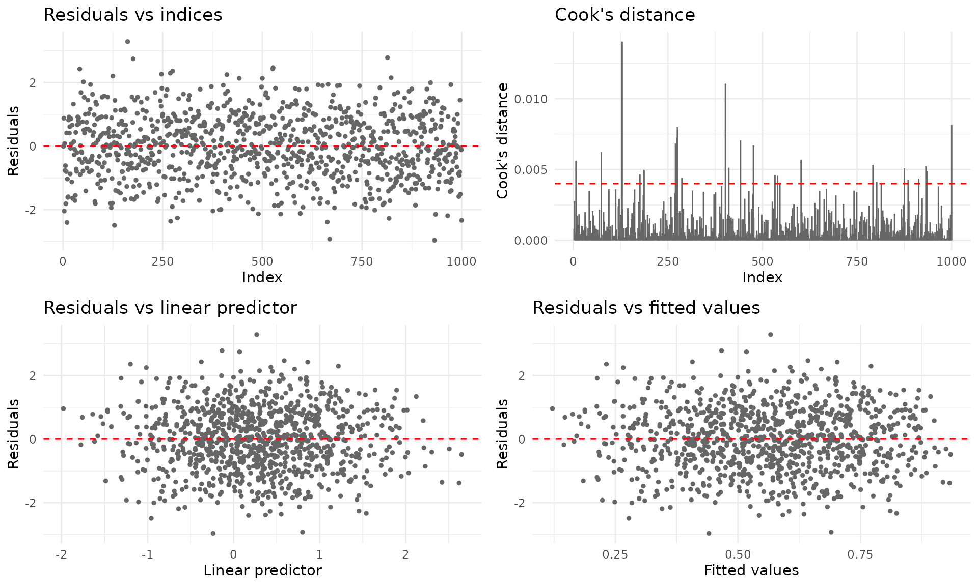

Predictions

# Fitted means
kbl10(
  data.frame(mu_hat = head(predict(fit_fixed, type = "response"))),
  digits = 4
)

mu_hat
0.3222
0.6343
0.5825
0.5148
0.5031
0.4115

# Conditional variance
kbl10(
  data.frame(var_hat = head(predict(fit_fixed, type = "variance"))),
  digits = 4
)

var_hat
0.1152
0.1224
0.1283
0.1317
0.1319
0.1277

# Quantile predictions
kbl10(predict(fit_fixed, type = "quantile", at = c(0.10, 0.25, 0.5, 0.75, 0.90)))

q_0.1	q_0.25	q_0.5	q_0.75	q_0.9
0.0007	0.0170	0.1779	0.6024	0.8964
0.0711	0.3148	0.7508	0.9675	0.9980
0.0435	0.2311	0.6578	0.9398	0.9947
0.0208	0.1444	0.5288	0.8860	0.9856
0.0181	0.1318	0.5060	0.8745	0.9833
0.0048	0.0565	0.3311	0.7601	0.9538
0.1348	0.4660	0.8689	0.9905	0.9997
0.1221	0.4392	0.8517	0.9880	0.9996
0.0319	0.1895	0.6011	0.9185	0.9915
0.0288	0.1777	0.5834	0.9111	0.9902

Confidence intervals

Wald confidence intervals based on the asymptotic normal approximation:

kbl10(confint(fit_fixed))

	2.5 %	97.5 %
(Intercept)	0.2215	0.3906
x1	-0.6921	-0.5145
x2	0.3554	0.5273
(phi)	0.0304	0.1894

kbl10(confint(fit_fixed, model = "mean"))

	2.5 %	97.5 %
(Intercept)	0.2215	0.3906
x1	-0.6921	-0.5145
x2	0.3554	0.5273

Censoring structure

The brs_cens() function provides a visual and tabular overview of the censoring types in the fitted model:

brs_cens(fit_fixed, gg = TRUE, inform = TRUE)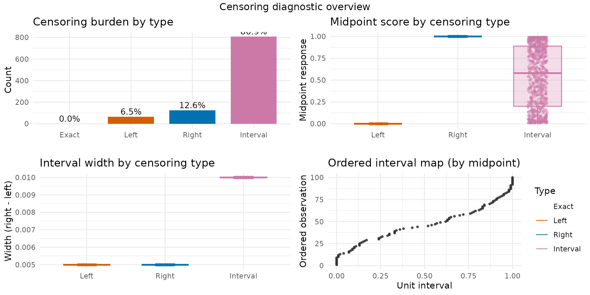

Example 2: Variable dispersion model

In many applications, the dispersion parameter $\phi$ may depend on covariates. The package supports variable-dispersion models using the Formula package notation: y ~ x1 + x2 | z1 + z2, where the terms after | define the linear predictor for $\phi$. The same brs_sim() function is used for fixed and variable dispersion; the second formula part activates the precision submodel in simulation.

Simulating data

set.seed(2222)
n <- 1000
dat_z <- data.frame(
  x1 = rnorm(n),
  x2 = rnorm(n),
  x3 = rbinom(n, size = 1, prob = 0.5),
  z1 = rnorm(n),
  z2 = rnorm(n)
)

sim_var <- brs_sim(
  formula = ~ x1 + x2 + x3 | z1 + z2,
  data = dat_z,
  beta = c(0.2, -0.6, 0.2, 0.2),
  zeta = c(0.2, -0.8, 0.6),
  link = "logit",
  link_phi = "logit",
  ncuts = 100,
  repar = 2
)

kbl10(head(sim_var, 10))

left	right	yt	y	delta	x1	x2	x3	z1	z2
0.265	0.275	0.27	27	3	-0.3381	-0.8235	0	0.0306	-1.1222
0.175	0.185	0.18	18	3	0.9392	-1.7563	0	0.1938	-0.2891
0.000	0.005	0.00	0	1	1.7377	-1.3148	1	-0.4283	0.3479
0.525	0.535	0.53	53	3	0.6963	-0.8196	0	0.3694	0.2811
0.085	0.095	0.09	9	3	0.4623	-0.1183	1	0.0553	-1.2184
0.955	0.965	0.96	96	3	-0.3151	-0.0648	1	0.7169	-0.5613
0.165	0.175	0.17	17	3	0.1927	-0.9985	0	-0.2222	0.4225
0.385	0.395	0.39	39	3	1.1307	0.6330	1	1.2509	-1.5492
0.005	0.015	0.01	1	3	1.9764	-0.4887	0	-1.8699	0.3679
0.515	0.525	0.52	52	3	1.2071	-1.3548	1	-0.2813	-1.6754

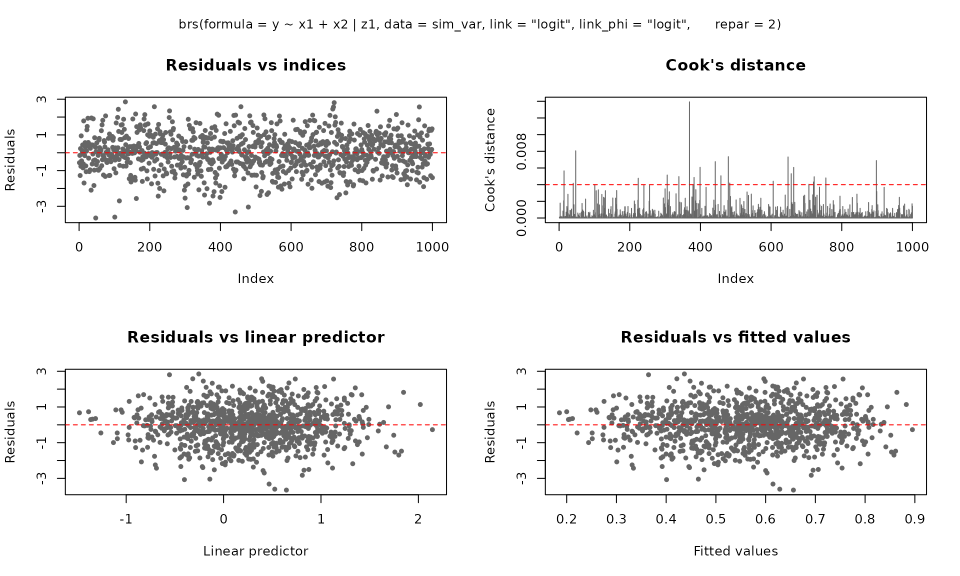
Fitting the model

fit_var <- brs(
  y ~ x1 + x2 | z1,
  data     = sim_var,
  link     = "logit",
  link_phi = "logit",
  repar    = 2
)
summary(fit_var)
#> 
#> Call:
#> brs(formula = y ~ x1 + x2 | z1, data = sim_var, link = "logit", 
#>     link_phi = "logit", repar = 2)
#> 
#> Quantile residuals:
#>     Min      1Q  Median      3Q     Max 
#> -3.6111 -0.6344  0.0131  0.6654  3.2463 
#> 
#> Coefficients (mean model with logit link):
#>             Estimate Std. Error z value Pr(>|z|)    
#> (Intercept)  0.27141    0.04245   6.394 1.62e-10 ***
#> x1          -0.54553    0.04375 -12.468  < 2e-16 ***
#> x2           0.17226    0.04141   4.160 3.18e-05 ***
#> ---
#> Signif. codes:  0 '***' 0.001 '**' 0.01 '*' 0.05 '.' 0.1 ' ' 1
#> 
#> Phi coefficients (precision model with logit link):
#>                   Estimate Std. Error z value Pr(>|z|)    
#> (phi)_(Intercept)  0.24653    0.04233   5.823 5.77e-09 ***
#> (phi)_z1          -0.72230    0.04507 -16.028  < 2e-16 ***
#> ---
#> Signif. codes:  0 '***' 0.001 '**' 0.01 '*' 0.05 '.' 0.1 ' ' 1
#> ---
#> Log-likelihood: -3922.2430 on 5 Df | AIC: 7854.4861 | BIC: 7879.0249 
#> Pseudo R-squared: 0.1159 
#> Number of iterations: 42 (BFGS) 
#> Censoring: 744 interval | 105 left | 151 right

Notice the (phi)_ prefix in the precision coefficient names, following the betareg convention.

Accessing coefficients by submodel

# Full parameter vector
round(coef(fit_var), 4)
#>       (Intercept)                x1                x2 (phi)_(Intercept) 
#>            0.2714           -0.5455            0.1723            0.2465 
#>          (phi)_z1 
#>           -0.7223

# Mean submodel only
round(coef(fit_var, model = "mean"), 4)
#> (Intercept)          x1          x2 
#>      0.2714     -0.5455      0.1723

# Precision submodel only
round(coef(fit_var, model = "precision"), 4)
#> (phi)_(Intercept)          (phi)_z1 
#>            0.2465           -0.7223

# Variance-covariance matrix for the mean submodel
kbl10(vcov(fit_var, model = "mean"))

	(Intercept)	x1	x2
(Intercept)	0.0018	-0.0001	0.0000
x1	-0.0001	0.0019	0.0000
x2	0.0000	0.0000	0.0017

Comparing link functions (variable dispersion)

links <- c("logit", "probit", "cauchit", "cloglog")
fits_var <- lapply(setNames(links, links), function(lnk) {
  brs(y ~ x1 + x2 | z1, data = sim_var, link = lnk, repar = 2)
})

# Estimates
est_var <- do.call(rbind, lapply(names(fits_var), function(lnk) {
  e <- brs_est(fits_var[[lnk]])
  e$link <- lnk
  e
}))
kbl10(est_var)

variable	estimate	se	z_value	p_value	ci_lower	ci_upper	link
(Intercept)	0.2714	0.0424	6.3938	0	0.1882	0.3546	logit
x1	-0.5455	0.0438	-12.4682	0	-0.6313	-0.4598	logit
x2	0.1723	0.0414	4.1599	0	0.0911	0.2534	logit
(phi)_(Intercept)	0.2465	0.0423	5.8234	0	0.1636	0.3295	logit
(phi)_z1	-0.7223	0.0451	-16.0277	0	-0.8106	-0.6340	logit
(Intercept)	0.1675	0.0260	6.4315	0	0.1165	0.2186	probit
x1	-0.3352	0.0262	-12.8011	0	-0.3865	-0.2839	probit
x2	0.1056	0.0253	4.1771	0	0.0561	0.1552	probit
(phi)_(Intercept)	0.2467	0.0423	5.8291	0	0.1638	0.3297	probit
(phi)_z1	-0.7229	0.0451	-16.0344	0	-0.8112	-0.6345	probit

# Goodness of fit
gof_var <- do.call(rbind, lapply(fits_var, brs_gof))
kbl10(gof_var)

	logLik	AIC	BIC	pseudo_r2
logit	-3922.243	7854.486	7879.025	0.1159
probit	-3922.227	7854.455	7878.994	0.1216
cauchit	-3923.161	7856.323	7880.862	0.0902
cloglog	-3922.296	7854.593	7879.132	0.0898

Diagnostics for variable dispersion

plot(fit_var)

Advanced analyst functions

The package includes analyst-facing helpers for uncertainty quantification, effect interpretation, score-scale communication, and predictive validation.

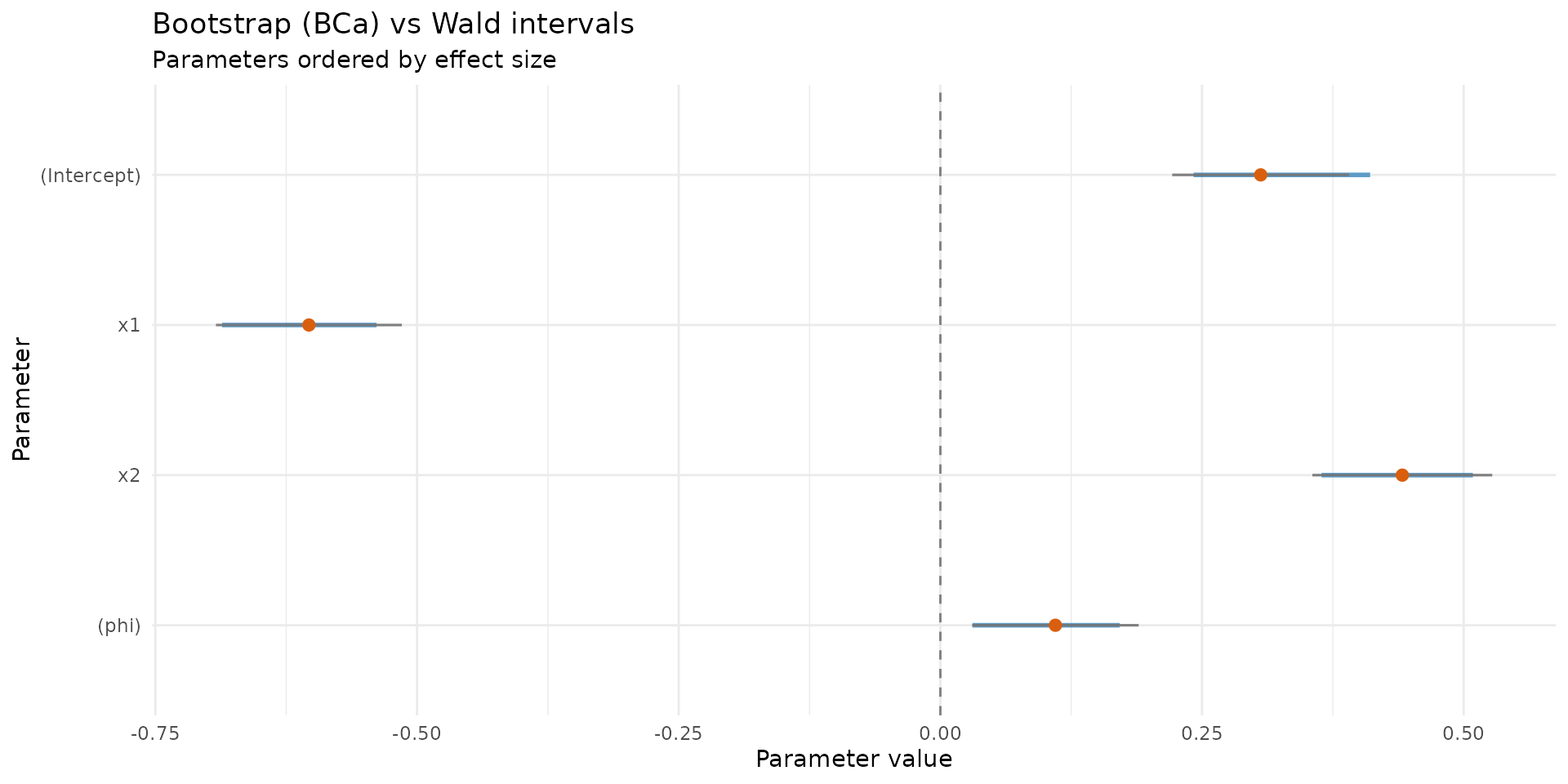
Parametric bootstrap confidence intervals

set.seed(101)
boot_ci <- brs_bootstrap(
  fit_fixed,
  R = 100,
  level = 0.95,
  ci_type = "bca",
  keep_draws = TRUE
)
kbl10(head(boot_ci, 10))

parameter	estimate	se_boot	ci_lower	ci_upper	mcse_lower	mcse_upper	wald_lower	wald_upper	level
(Intercept)	0.3060	0.0410	0.2420	0.4106	0.0058	0.0137	0.2215	0.3906	0.95
x1	-0.6033	0.0424	-0.6863	-0.5387	0.0059	0.0045	-0.6921	-0.5145	0.95
x2	0.4413	0.0423	0.3641	0.5088	0.0100	0.0034	0.3554	0.5273	0.95
(phi)	0.1099	0.0396	0.0307	0.1714	0.0093	0.0039	0.0304	0.1894	0.95

autoplot.brs_bootstrap(
  boot_ci,
  type = "ci_forest",
  title = "Bootstrap (BCa) vs Wald intervals"
)

Average marginal effects (AME)

set.seed(202)
ame <- brs_marginaleffects(
  fit_fixed,
  model = "mean",
  type = "response",
  interval = TRUE,
  n_sim = 120,
  keep_draws = TRUE
)
kbl10(ame)

variable	ame	std.error	ci.lower	ci.upper	model	type	n
x1	-0.1321	0.0088	-0.1473	-0.1123	mean	response	1000
x2	0.0966	0.0093	0.0798	0.1140	mean	response	1000

autoplot.brs_marginaleffects(ame, type = "forest")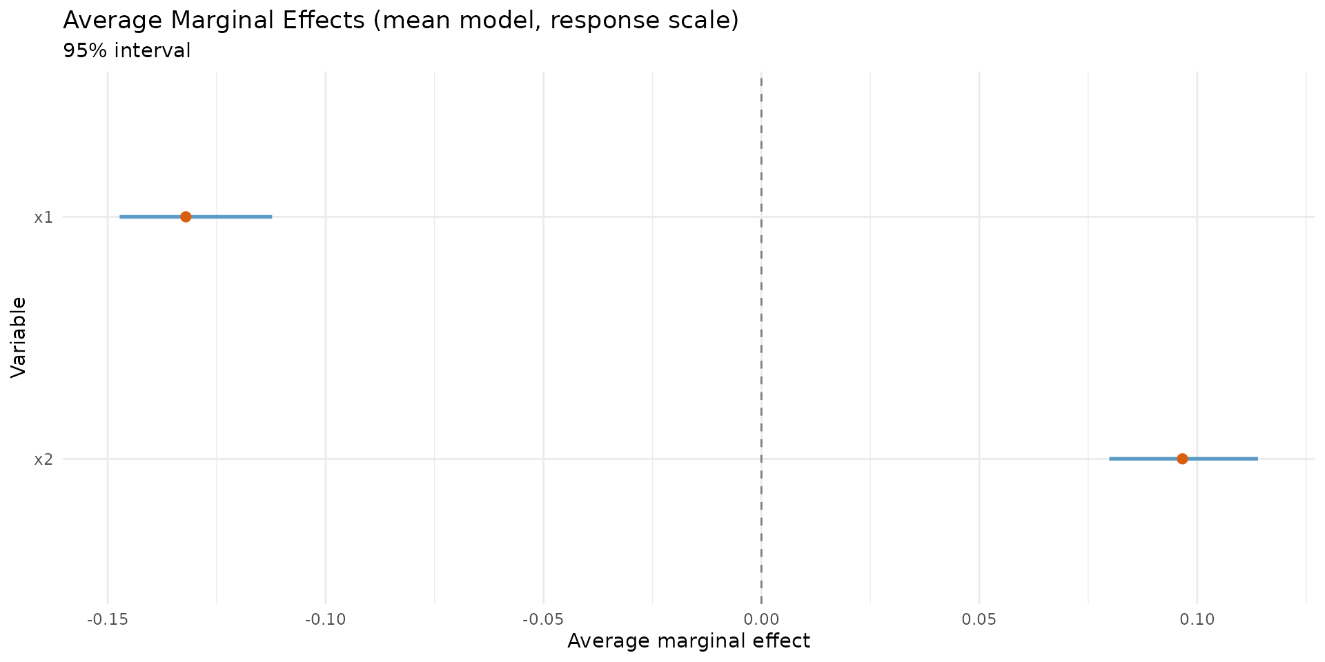

Score probabilities on the original scale

prob_scores <- brs_predict_scoreprob(fit_fixed, scores = 0:10)
kbl10(prob_scores[1:6, 1:6])

score_0	score_1	score_2	score_3	score_4	score_5
0.1754	0.0657	0.0386	0.0288	0.0235	0.0201
0.0218	0.0190	0.0139	0.0117	0.0104	0.0095
0.0320	0.0249	0.0176	0.0145	0.0127	0.0115
0.0516	0.0342	0.0230	0.0185	0.0159	0.0142
0.0559	0.0360	0.0240	0.0192	0.0165	0.0146
0.1016	0.0509	0.0318	0.0246	0.0206	0.0180

kbl10(
  data.frame(row_sum = rowSums(prob_scores)[1:6]),
  digits = 4
)

row_sum
0.4263
0.1260
0.1605
0.2141
0.2245
0.3163

Repeated k-fold cross-validation

set.seed(303) # For cross-validation reproducibility
cv_res <- brs_cv(
  y ~ x1 + x2,
  data = sim_fixed,
  k = 5,
  repeats = 5,
  repar = 2,
)
kbl10(cv_res)

repeat	fold	n_train	n_test	log_score	rmse_yt	mae_yt	converged	error
1	1	800	200	-4.0713	0.3472	0.3019	TRUE	NA
1	2	800	200	-3.9984	0.3451	0.3019	TRUE	NA
1	3	800	200	-3.9235	0.3395	0.2997	TRUE	NA
1	4	800	200	-4.0902	0.3311	0.2874	TRUE	NA
1	5	800	200	-4.1125	0.3420	0.2958	TRUE	NA
2	1	800	200	-4.0795	0.3270	0.2892	TRUE	NA
2	2	800	200	-4.2062	0.3504	0.2972	TRUE	NA
2	3	800	200	-4.1858	0.3248	0.2818	TRUE	NA
2	4	800	200	-3.8729	0.3457	0.3036	TRUE	NA
2	5	800	200	-3.8752	0.3578	0.3159	TRUE	NA

kbl10(
  data.frame(
    metric = c("log_score", "rmse_yt", "mae_yt"),
    mean = c(
      mean(cv_res$log_score, na.rm = TRUE),
      mean(cv_res$rmse_yt, na.rm = TRUE),
      mean(cv_res$mae_yt, na.rm = TRUE)
    )
  ),
  digits = 4
)

metric	mean
log_score	-4.0404
rmse_yt	0.3409
mae_yt	0.2974

S3 methods reference

The following standard S3 methods are available for objects of class "brs":

Method	Description
print()	Compact display of call and coefficients
summary()	Detailed output with Wald tests and goodness-of-fit
coef(model=)	Extract coefficients (full, mean, or precision)
vcov(model=)	Variance-covariance matrix (full, mean, or precision)
confint(model=)	Wald confidence intervals
logLik()	Log-likelihood value
AIC(), BIC()	Information criteria
nobs()	Number of observations
formula()	Model formula
model.matrix(model=)	Design matrix (mean or precision)
fitted()	Fitted mean values
residuals(type=)	Residuals: response, pearson, rqr, weighted, sweighted
predict(type=)	Predictions: response, link, precision, variance, quantile
plot(gg=)	Diagnostic plots (base R or ggplot2)

Reparameterizations

The package supports three reparameterizations of the beta distribution, controlled by the repar argument:

Direct (repar = 0): Shape parameters $a=\mu$ and $b=\phi$ are used directly. This is rarely used in practice.

Precision (repar = 1, Ferrari & Cribari-Neto, 2004): The mean $\mu\in(0,1)$ and precision $\phi>0$ yield $a=\mu\phi$ and $b=(1-\mu)\phi$. Higher $\phi$ means less variability.

Mean–variance (repar = 2): The mean $\mu\in(0,1)$ and dispersion $\phi\in(0,1)$ yield $a=\mu(1-\phi)/\phi$ and $b=(1-\mu)(1-\phi)/\phi$. Here $\phi$ acts as a coefficient of variation: smaller $\phi$ means less variability.

# Precision parameterization: mu = 0.5, phi = 10 (high precision)
brs_repar(mu = 0.5, phi = 10, repar = 1)
#>   shape1 shape2
#> 1      5      5

# Mean-variance parameterization: mu = 0.5, phi = 0.1 (low dispersion)
brs_repar(mu = 0.5, phi = 0.1, repar = 2)
#>   shape1 shape2
#> 1    4.5    4.5

References

• Ferrari, S. L. P., and Cribari-Neto, F. (2004). Beta regression for modelling rates and proportions. Journal of Applied Statistics, 31(7), 799–815. DOI: 10.1080/0266476042000214501. Validated online via: https://doi.org/10.1080/0266476042000214501.

• Smithson, M., and Verkuilen, J. (2006). A better lemon squeezer? Maximum-likelihood regression with beta-distributed dependent variables. Psychological Methods, 11(1), 54–71. DOI: 10.1037/1082-989X.11.1.54. Validated online via: https://doi.org/10.1037/1082-989X.11.1.54.

• Hawker, G. A., Mian, S., Kendzerska, T., and French, M. (2011). Measures of adult pain: Visual Analog Scale for Pain (VAS Pain), Numeric Rating Scale for Pain (NRS Pain), McGill Pain Questionnaire (MPQ), Short-Form McGill Pain Questionnaire (SF-MPQ), Chronic Pain Grade Scale (CPGS), Short Form-36 Bodily Pain Scale (SF-36 BPS), and Measure of Intermittent and Constant Osteoarthritis Pain (ICOAP). Arthritis Care and Research, 63(S11), S240–S252. DOI: 10.1002/acr.20543. Validated online via: https://doi.org/10.1002/acr.20543.

• Hjermstad, M. J., Fayers, P. M., Haugen, D. F., et al. (2011). Studies comparing numerical rating scales, verbal rating scales, and visual analogue scales for assessment of pain intensity in adults: a systematic literature review. Journal of Pain and Symptom Management, 41(6), 1073–1093. DOI: 10.1016/j.jpainsymman.2010.08.016. Validated online via: https://doi.org/10.1016/j.jpainsymman.2010.08.016.