Analyst Tools for betaregscale • betaregscale

Overview

This vignette presents analyst-oriented tools added to betaregscale for post-estimation workflows:

brs_table(): model comparison tables.
brs_marginaleffects(): average marginal effects (AME).
brs_predict_scoreprob(): probabilities on the original score scale.
autoplot.brs(): ggplot2 diagnostics.
brs_cv(): repeated k-fold cross-validation.

The examples use bounded scale data under the interval-censored beta regression framework implemented in the package.

library(betaregscale)

Mathematical foundations

Complete likelihood by censoring type

For each observation $i$ , let $\delta_i\in\{0,1,2,3\}$ indicate exact, left-censored, right-censored, or interval-censored status. With beta CDF $F(\cdot)$ , beta density $f(\cdot)$ , and interval endpoints $[l_i,u_i]$ , the contribution is:

$L_i(\theta)= \begin{cases} f(y_i; a_i, b_i), & \delta_i=0,\\ F(u_i; a_i, b_i), & \delta_i=1,\\ 1 - F(l_i; a_i, b_i), & \delta_i=2,\\ F(u_i; a_i, b_i)-F(l_i; a_i, b_i), & \delta_i=3. \end{cases}$

This is the basis for fitting, prediction, and validation metrics.

Model-comparison metrics

brs_table() reports:

$\log L(\hat\theta)$ ,
$AIC=-2\log L(\hat\theta)+2k$ ,
$BIC=-2\log L(\hat\theta)+k\log n$ ,

where $k$ is the number of estimated parameters and $n$ is the sample size.

Average marginal effects (AME)

brs_marginaleffects() computes AME by finite differences:

$\mathrm{AME}_j=\frac{1}{n}\sum_{i=1}^n\frac{\hat g_i(x_{ij}+h)-\hat g_i(x_{ij})}{h},$

with $\hat g_i$ on the requested prediction scale (response or link). For binary covariates $x_j\in\{0,1\}$ , it uses the discrete contrast $\hat g(x_j=1)-\hat g(x_j=0)$ .

Score-scale probabilities

For integer scores $s\in\{0,\dots,K\}$ , brs_predict_scoreprob() computes:

$P(Y=s)= \begin{cases} F(\mathrm{lim}/K), & s=0,\\ 1-F((K-\mathrm{lim})/K), & s=K,\\ F((s+\mathrm{lim})/K)-F((s-\mathrm{lim})/K), & 1\le s\le K-1. \end{cases}$

These probabilities are directly aligned with interval geometry on the original instrument scale.

Cross-validation log score

In brs_cv(), fold-level predictive quality includes:

$\mathrm{log\_score}=\frac{1}{n_{test}}\sum_{i \in test}\log(p_i),$

where $p_i$ is the predictive contribution from the same censoring-rule piecewise definition shown above.

It also reports:

$\mathrm{RMSE}_{yt}=\sqrt{\frac{1}{n_{test}}\sum(y_{t,i}-\hat\mu_i)^2}, \qquad \mathrm{MAE}_{yt}=\frac{1}{n_{test}}\sum|y_{t,i}-\hat\mu_i|.$

Reproducible workflow

1) Simulate data and fit candidate models

set.seed(2026)
n <- 220
d <- data.frame(
  x1 = rnorm(n),
  x2 = rnorm(n),
  z1 = rnorm(n)
)

sim <- brs_sim(
  formula = ~ x1 + x2 | z1,
  data = d,
  beta = c(0.20, -0.45, 0.25),
  zeta = c(0.15, -0.30),
  ncuts = 100,
  repar = 2
)

fit_fixed <- brs(y ~ x1 + x2, data = sim, repar = 2)
fit_var <- brs(y ~ x1 + x2 | z1, data = sim, repar = 2)

2) Compare models in one table

tab <- brs_table(
  fixed = fit_fixed,
  variable = fit_var,
  sort_by = "AIC"
)
kbl10(tab)

model	nobs	npar	logLik	AIC	BIC	pseudo_r2	exact	left	right	interval	prop_exact	prop_left	prop_right	prop_interval
variable	220	5	-931.8646	1873.729	1890.697	0.1381	0	8	22	190	0	0.0364	0.1	0.8636
fixed	220	4	-939.3243	1886.649	1900.223	0.1381	0	8	22	190	0	0.0364	0.1	0.8636

3) Estimate average marginal effects

set.seed(2026) # For marginal effects simulation
me_mean <- brs_marginaleffects(
  fit_var,
  model = "mean",
  type = "response",
  interval = TRUE,
  n_sim = 120
)
kbl10(me_mean)

variable	ame	std.error	ci.lower	ci.upper	model	type	n
x1	-0.1035	0.0178	-0.1339	-0.0675	mean	response	220
x2	0.0734	0.0188	0.0360	0.1071	mean	response	220


set.seed(2026) # Reset seed for reproducibility
me_precision <- brs_marginaleffects(
  fit_var,
  model = "precision",
  type = "link",
  interval = TRUE,
  n_sim = 120
)
kbl10(me_precision)

variable	ame	std.error	ci.lower	ci.upper	model	type	n
z1	-0.3361	0.0835	-0.4781	-0.1413	precision	link	220

4) Predict score probabilities

P <- brs_predict_scoreprob(fit_var, scores = 0:10)
dim(P)
#> [1] 220  11
kbl10(P[1:6, 1:5])

score_0	score_1	score_2	score_3	score_4
0.0146	0.0178	0.0146	0.0130	0.0121
0.0215	0.0228	0.0178	0.0155	0.0141
0.0465	0.0318	0.0216	0.0175	0.0151
0.0731	0.0371	0.0233	0.0181	0.0152
0.0076	0.0105	0.0090	0.0083	0.0078
0.0050	0.0050	0.0039	0.0034	0.0030

kbl10(
  data.frame(row_sum = rowSums(P)),
  digits = 4
)

row_sum
0.1344
0.1614
0.2001
0.2313
0.0856
0.0354
0.0295
0.0994
0.1024
0.1312

rowSums(P) should be close to 1 (up to numerical tolerance and score subset selection).

5) ggplot2 diagnostics

autoplot.brs(fit_var, type = "calibration")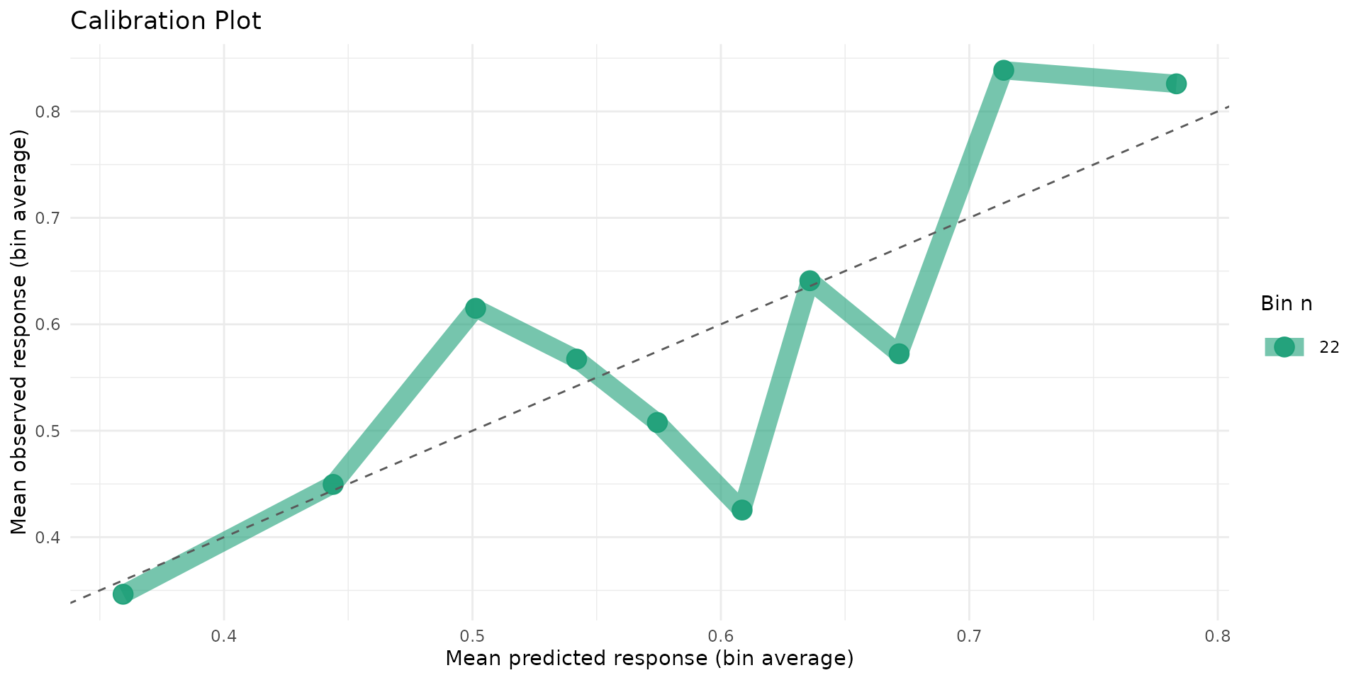

autoplot.brs(fit_var, type = "score_dist", scores = 0:20)

autoplot.brs(fit_var, type = "cdf", max_curves = 4)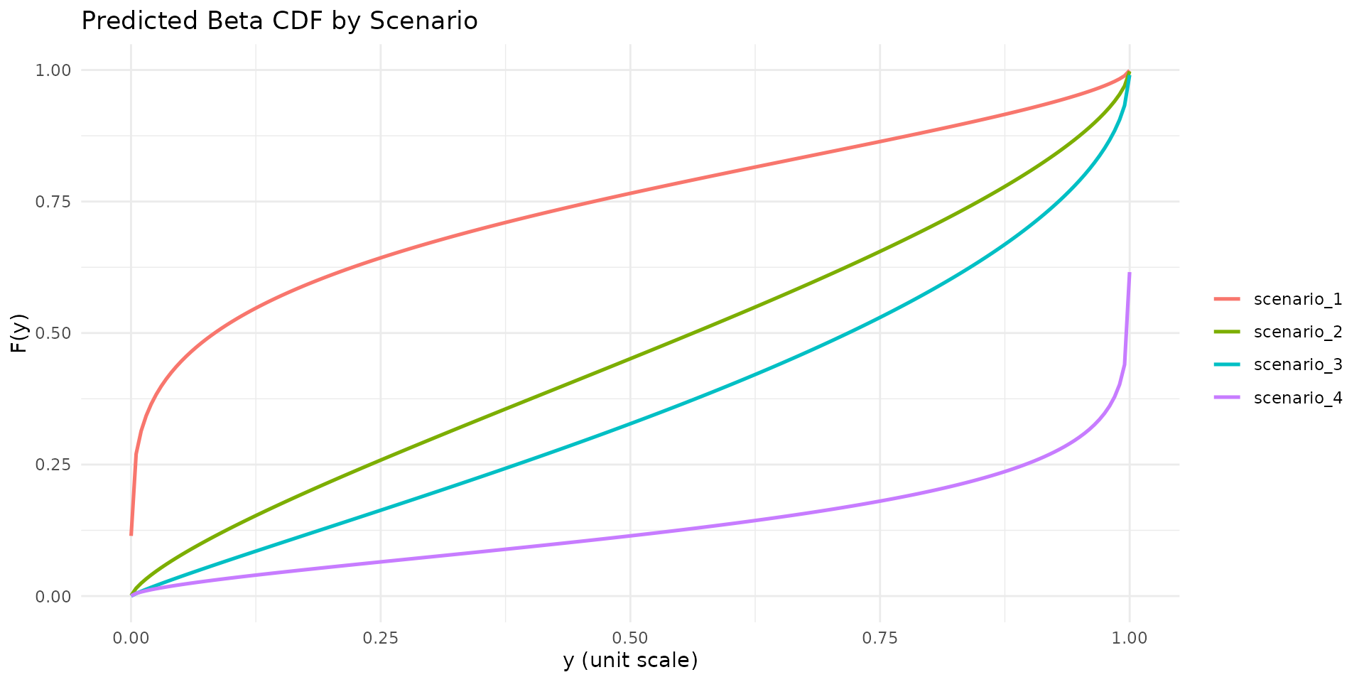

autoplot.brs(fit_var, type = "residuals_by_delta", residual_type = "rqr")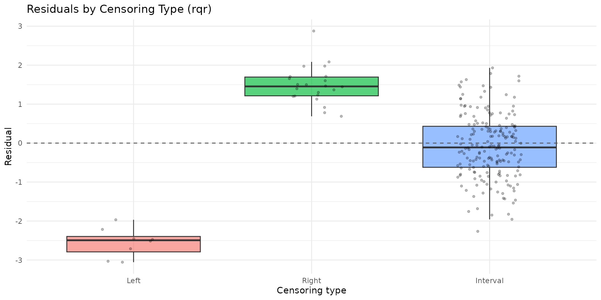

6) Repeated k-fold cross-validation

set.seed(2026) # For cross-validation reproducibility
cv_res <- brs_cv(
  y ~ x1 + x2 | z1,
  data = sim,
  k = 3,
  repeats = 1,
  repar = 2
)

kbl10(cv_res)

repeat	fold	n_train	n_test	log_score	rmse_yt	mae_yt	converged	error
1	1	146	74	-4.3077	0.3215	0.2862	TRUE	NA
1	2	147	73	-4.3171	0.3449	0.3032	TRUE	NA
1	3	147	73	-4.1676	0.3454	0.3022	TRUE	NA

kbl10(
  data.frame(
    metric = c("log_score", "rmse_yt", "mae_yt"),
    mean = colMeans(cv_res[, c("log_score", "rmse_yt", "mae_yt")], na.rm = TRUE)
  ),
  digits = 4
)

	metric	mean
log_score	log_score	-4.2641
rmse_yt	rmse_yt	0.3373
mae_yt	mae_yt	0.2972

Practical interpretation

Prefer the model with the lower AIC/BIC and better predictive log_score.
Use AME on the response scale to communicate the expected change in mean score (on the unit interval) resulting from small covariate shifts.
Use score probabilities to translate model outputs back to clinically interpretable scale categories.
Inspect calibration and residual-by-censoring plots before proceeding with statistical inference.

References

Ferrari, S. L. P., and Cribari-Neto, F. (2004). Beta regression for modelling rates and proportions. Journal of Applied Statistics, 31(7), 799-815. DOI: 10.1080/0266476042000214501. Validated online via: https://doi.org/10.1080/0266476042000214501.
Hawker, G. A., Mian, S., Kendzerska, T., and French, M. (2011). Measures of adult pain: VAS, NRS, MPQ, SF-MPQ, CPGS, SF-36 BPS, and ICOAP. Arthritis Care and Research, 63(S11), S240-S252. DOI: 10.1002/acr.20543. Validated online via: https://doi.org/10.1002/acr.20543.
Hjermstad, M. J., Fayers, P. M., Haugen, D. F., et al. (2011). Comparing NRS, VRS, and VAS pain scales in adults: a systematic review. Journal of Pain and Symptom Management, 41(6), 1073-1093. DOI: 10.1016/j.jpainsymman.2010.08.016. Validated online via: https://doi.org/10.1016/j.jpainsymman.2010.08.016.