ggplot2 autoplot for brs models

Produces ggplot2 diagnostics tailored to interval-censored scale models.

Usage

# S3 method for class 'brs'
autoplot(
  object,
  type = c("calibration", "score_dist", "cdf", "residuals_by_delta", "all"),
  bins = 10L,
  scores = NULL,
  newdata = NULL,
  n_grid = 200L,
  max_curves = 6L,
  residual_type = "rqr",
  title = NULL,
  xlab = NULL,
  ylab = NULL,
  ncol = 2L,
  theme = ggplot2::theme_minimal(),
  ...
)

Arguments

object: A fitted "brs" object.
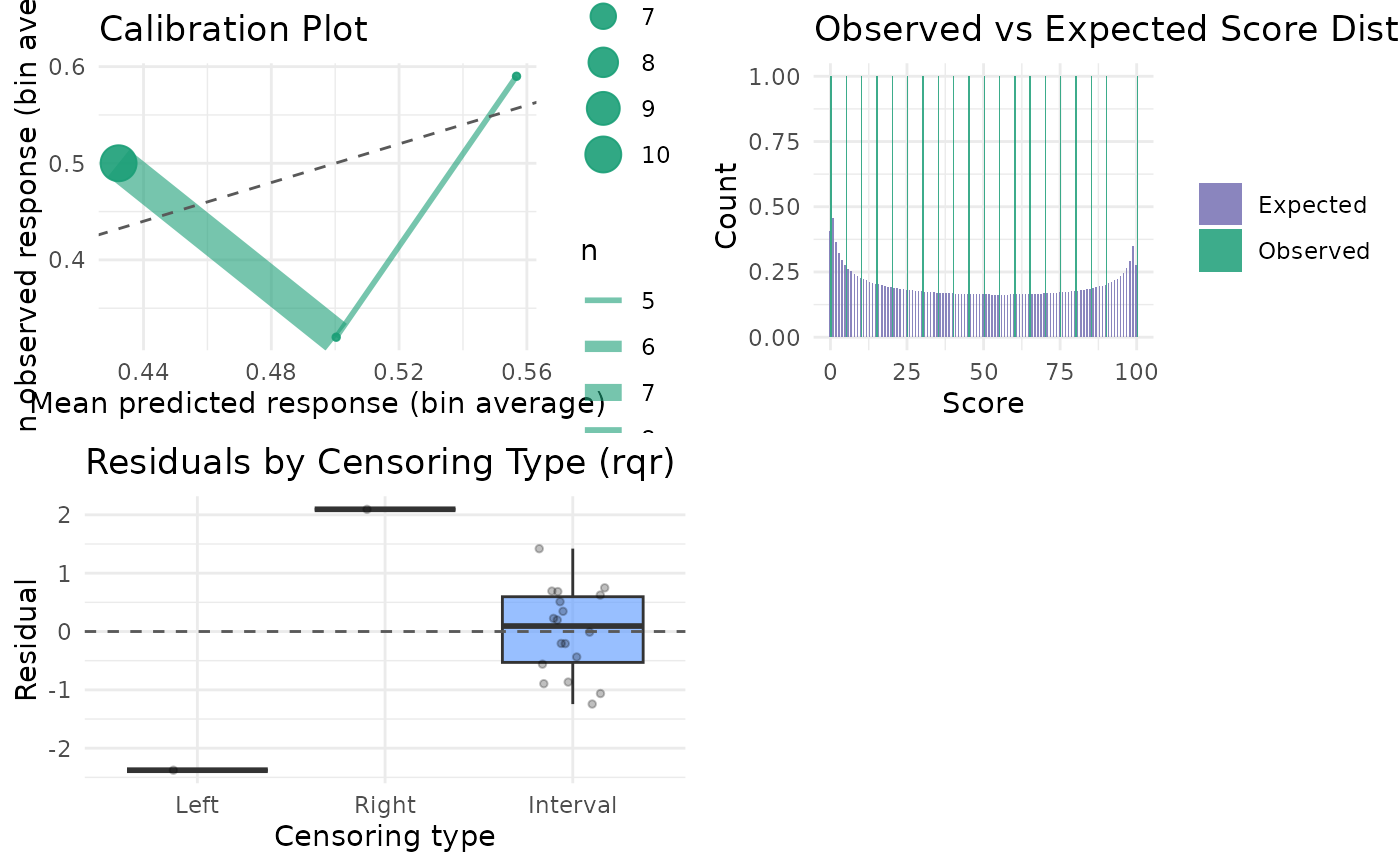
type: Plot type: "calibration", "score_dist", "cdf", "residuals_by_delta", or "all" (produces all panels in a single grid).
bins: Number of bins for "calibration".
scores: Optional integer vector of scores for "score_dist". Defaults to all scores from 0 to ncuts.
newdata: Optional data frame of covariate scenarios for "cdf".
n_grid: Number of points on \((0,1)\) used to draw CDF curves.
max_curves: Maximum number of CDF curves shown when newdata is not provided.
residual_type: Residual type for "residuals_by_delta"; passed to residuals.brs.
title: Optional character: override the plot title via ggplot2::labs(title = ...). Ignored when type = "all".
xlab: Optional character: override the x-axis label. Ignored when type = "all".
ylab: Optional character: override the y-axis label. Ignored when type = "all".
ncol: Number of columns for the grid when type = "all". Defaults to 2.
theme: A ggplot2 theme object (e.g., ggplot2::theme_bw()) or a theme function. Applied to every panel. Defaults to ggplot2::theme_minimal().
...: Additional arguments forwarded to ggplot2::theme() and applied on top of theme. Use named theme element arguments, e.g. legend.position = "none".

Value

A ggplot2 object.

Details

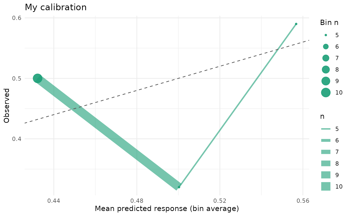
type = "calibration" bins predictions and compares mean observed vs mean predicted response in each bin.

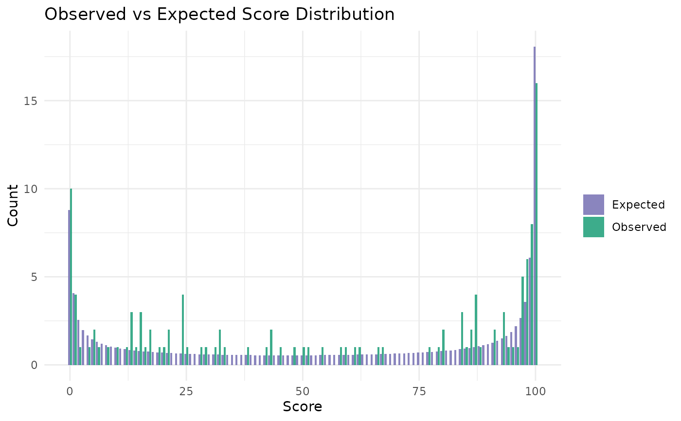
type = "score_dist" compares observed score frequencies against expected frequencies implied by the fitted beta interval model.

References

Lopes, J. E. (2023). Modelos de regressao beta para dados de escala. Master's dissertation, Universidade Federal do Parana, Curitiba. URI: https://hdl.handle.net/1884/86624.

Hawker, G. A., Mian, S., Kendzerska, T., and French, M. (2011). Measures of adult pain: Visual Analog Scale for Pain (VAS Pain), Numeric Rating Scale for Pain (NRS Pain), McGill Pain Questionnaire (MPQ), Short-Form McGill Pain Questionnaire (SF-MPQ), Chronic Pain Grade Scale (CPGS), Short Form-36 Bodily Pain Scale (SF-36 BPS), and Measure of Intermittent and Constant Osteoarthritis Pain (ICOAP). Arthritis Care and Research, 63(S11), S240-S252. doi:10.1002/acr.20543

Hjermstad, M. J., Fayers, P. M., Haugen, D. F., et al. (2011). Studies comparing Numerical Rating Scales, Verbal Rating Scales, and Visual Analogue Scales for assessment of pain intensity in adults: a systematic literature review. Journal of Pain and Symptom Management, 41(6), 1073-1093. doi:10.1016/j.jpainsymman.2010.08.016

Examples

# \donttest{
dat <- data.frame(
  y = c(
    0, 5, 20, 50, 75, 90, 100, 30, 60, 45,
    10, 40, 55, 70, 85, 25, 35, 65, 80, 15
  ),
  x1 = rep(c(1, 2), 10),
  x2 = rep(c(0, 0, 1, 1), 5)
)
prep <- brs_prep(dat, ncuts = 100)
#> brs_prep: n = 20 | exact = 0, left = 1, right = 1, interval = 18
fit <- brs(y ~ x1 + x2, data = prep)
ggplot2::autoplot(fit, type = "calibration")

ggplot2::autoplot(fit,
  type = "calibration",
  title = "My calibration", ylab = "Observed"
)

ggplot2::autoplot(fit, type = "all")

# }