Mixed-Effects Beta Interval Regression with brsmm

Overview

brsmm() extends brs() to clustered data by adding a Gaussian random intercept in the mean submodel while preserving the interval-censored beta likelihood for scale-derived outcomes.

This vignette covers:

full model mathematics;
estimation by marginal maximum likelihood (Laplace approximation);
practical use of all current brsmm methods;
inferential and validation workflows, including parameter recovery.

library(betaregscale)

Mathematical model

Assume observations $i = 1, \dots, n_j$ within groups $j = 1, \dots, G$ , with random intercept $b_j \sim \mathcal{N}(0,\sigma_b^2)$ .

Linear predictors

$\eta_{\mu,ij} = x_{ij}^\top \beta + b_j, \qquad \eta_{\phi,ij} = z_{ij}^\top \gamma$

$\mu_{ij} = g^{-1}(\eta_{\mu,ij}), \qquad \phi_{ij} = h^{-1}(\eta_{\phi,ij})$

with $g(\cdot)$ and $h(\cdot)$ chosen by link and link_phi.

Beta parameterization

For each $(\mu_{ij}, \phi_{ij})$ , repar maps to beta shape parameters $(a_{ij}, b_{ij})$ via brs_repar().

Conditional contribution by censoring type

Each observation contributes:

$L_{ij}(b_j;\theta)= \begin{cases} f(y_{ij}; a_{ij}, b_{ij}), & \delta_{ij}=0\\ F(u_{ij}; a_{ij}, b_{ij}), & \delta_{ij}=1\\ 1 - F(l_{ij}; a_{ij}, b_{ij}), & \delta_{ij}=2\\ F(u_{ij}; a_{ij}, b_{ij}) - F(l_{ij}; a_{ij}, b_{ij}), & \delta_{ij}=3 \end{cases}$

where $l_{ij},u_{ij}$ are interval endpoints on $(0,1)$ , $f(\cdot)$ is beta density, and $F(\cdot)$ is beta CDF.

Group marginal likelihood

$L_j(\theta)=\int_{\mathbb{R}} \prod_{i=1}^{n_j} L_{ij}(b_j;\theta)\, \varphi(b_j;0,\sigma_b^2)\,db_j$

$\ell(\theta)=\sum_{j=1}^G \log L_j(\theta)$

Laplace approximation used by `brsmm()`

Define $Q_j(b)=\sum_{i=1}^{n_j}\log L_{ij}(b;\theta)+\log\varphi(b;0,\sigma_b^2)$ and $\hat b_j=\arg\max_b Q_j(b)$ , with curvature $H_j=-Q_j''(\hat b_j)$ . Then

$\log L_j(\theta) \approx Q_j(\hat b_j) + \frac{1}{2}\log(2\pi) - \frac{1}{2}\log(H_j).$

brsmm() maximizes the approximated $\ell(\theta)$ with stats::optim(), and computes group-level posterior modes $\hat b_j$ and local standard deviations from the local curvature.

Simulating clustered scale data

The next helper simulates data from a known mixed model to illustrate fitting, inference, and recovery checks.

sim_brsmm_data <- function(seed = 3501L, g = 24L, ni = 12L,
                           beta = c(0.20, 0.65),
                           gamma = c(-0.15),
                           sigma_b = 0.55) {
  set.seed(seed)
  id <- factor(rep(seq_len(g), each = ni))
  n <- length(id)
  x1 <- rnorm(n)

  b_true <- rnorm(g, mean = 0, sd = sigma_b)
  eta_mu <- beta[1] + beta[2] * x1 + b_true[as.integer(id)]
  eta_phi <- rep(gamma[1], n)

  mu <- plogis(eta_mu)
  phi <- plogis(eta_phi)
  shp <- brs_repar(mu = mu, phi = phi, repar = 2)
  y <- round(stats::rbeta(n, shp$shape1, shp$shape2) * 100)

  list(
    data = data.frame(y = y, x1 = x1, id = id),
    truth = list(beta = beta, gamma = gamma, sigma_b = sigma_b, b = b_true)
  )
}

sim <- sim_brsmm_data()
str(sim$data)
#> 'data.frame':    288 obs. of  3 variables:
#>  $ y : num  18 29 12 43 56 55 3 21 4 4 ...
#>  $ x1: num  -0.3677 -2.0069 -0.0469 -0.2468 0.7634 ...
#>  $ id: Factor w/ 24 levels "1","2","3","4",..: 1 1 1 1 1 1 1 1 1 1 ...

Fitting `brsmm()`

fit_mm <- brsmm(
  y ~ x1,
  random = ~ 1 | id,
  data = sim$data,
  repar = 2,
  int_method = "laplace",
  method = "BFGS",
  control = list(maxit = 1000)
)

fit_mm
#> 
#> Call:
#> brsmm(formula = y ~ x1, random = ~1 | id, data = sim$data, repar = 2, 
#>     int_method = "laplace", method = "BFGS", control = list(maxit = 1000))
#> 
#> Mixed beta interval model (Laplace)
#> Observations: 288  | Groups: 24 
#> Log-likelihood: -1231.3848 
#> Random SD: 0.4303 
#> Convergence code: 0

Core methods

Coefficients and random effects

coef(fit_mm, model = "random") is on the optimizer scale ( $\log \sigma_b$ ); use exp() to report $\sigma_b$ .

coef(fit_mm, model = "full")
#>       (Intercept)                x1 (phi)_(Intercept)           (sd)_id 
#>        0.01051336        0.62964563       -0.13626654       -0.84336505
coef(fit_mm, model = "mean")
#> (Intercept)          x1 
#>  0.01051336  0.62964563
coef(fit_mm, model = "precision")
#> (phi)_(Intercept) 
#>        -0.1362665
coef(fit_mm, model = "random")
#>   (sd)_id 
#> -0.843365
exp(coef(fit_mm, model = "random"))
#>   (sd)_id 
#> 0.4302602
head(ranef.brsmm(fit_mm))
#>           1           2           3           4           5           6 
#> -0.37076507  0.45544785 -0.17418739 -0.45940282  0.02481745  0.42957923

Variance-covariance, summary and likelihood criteria

vc <- vcov(fit_mm)
dim(vc)
#> [1] 4 4

sm <- summary(fit_mm)
sm
#> 
#> Call:
#> brsmm(formula = y ~ x1, random = ~1 | id, data = sim$data, repar = 2, 
#>     int_method = "laplace", method = "BFGS", control = list(maxit = 1000))
#> 
#> Mixed beta interval model (Laplace)
#> Observations: 288  | Groups: 24 
#> logLik =-1231.3848 | AIC =2470.7696 | BIC =2485.4215
#> 
#>                   Estimate Std. Error z value Pr(>|z|)    
#> (Intercept)        0.01051    0.05998   0.175   0.8609    
#> x1                 0.62965    0.08650   7.280 3.35e-13 ***
#> (phi)_(Intercept) -0.13627    0.07704  -1.769   0.0769 .  
#> (sd)_id           -0.84337    0.26045  -3.238   0.0012 ** 
#> ---
#> Signif. codes:  0 '***' 0.001 '**' 0.01 '*' 0.05 '.' 0.1 ' ' 1

logLik(fit_mm)
#> 'log Lik.' -1231.385 (df=4)
AIC(fit_mm)
#> [1] 2470.77
BIC(fit_mm)
#> [1] 2485.421
nobs(fit_mm)
#> [1] 288

Fitted values, prediction and residuals

head(fitted(fit_mm, type = "mu"))
#> [1] 0.3562286 0.1646701 0.4037733 0.3738710 0.5300708 0.3169583
head(fitted(fit_mm, type = "phi"))
#> [1] 0.465986 0.465986 0.465986 0.465986 0.465986 0.465986

head(predict(fit_mm, type = "response"))
#>         1         1         1         1         1         1 
#> 0.3562286 0.1646701 0.4037733 0.3738710 0.5300708 0.3169583
head(predict(fit_mm, type = "link"))
#>          1          1          1          1          1          1 
#> -0.5917708 -1.6238828 -0.3897673 -0.5156458  0.1204284 -0.7677855
head(predict(fit_mm, type = "precision"))
#> [1] 0.465986 0.465986 0.465986 0.465986 0.465986 0.465986
head(predict(fit_mm, type = "variance"))
#> [1] 0.10686447 0.06409816 0.11218166 0.10908334 0.11607513 0.10088398

head(residuals(fit_mm, type = "response"))
#> [1] -0.17622865  0.12532992 -0.28377333  0.05612904  0.02992923  0.23304166
head(residuals(fit_mm, type = "pearson"))
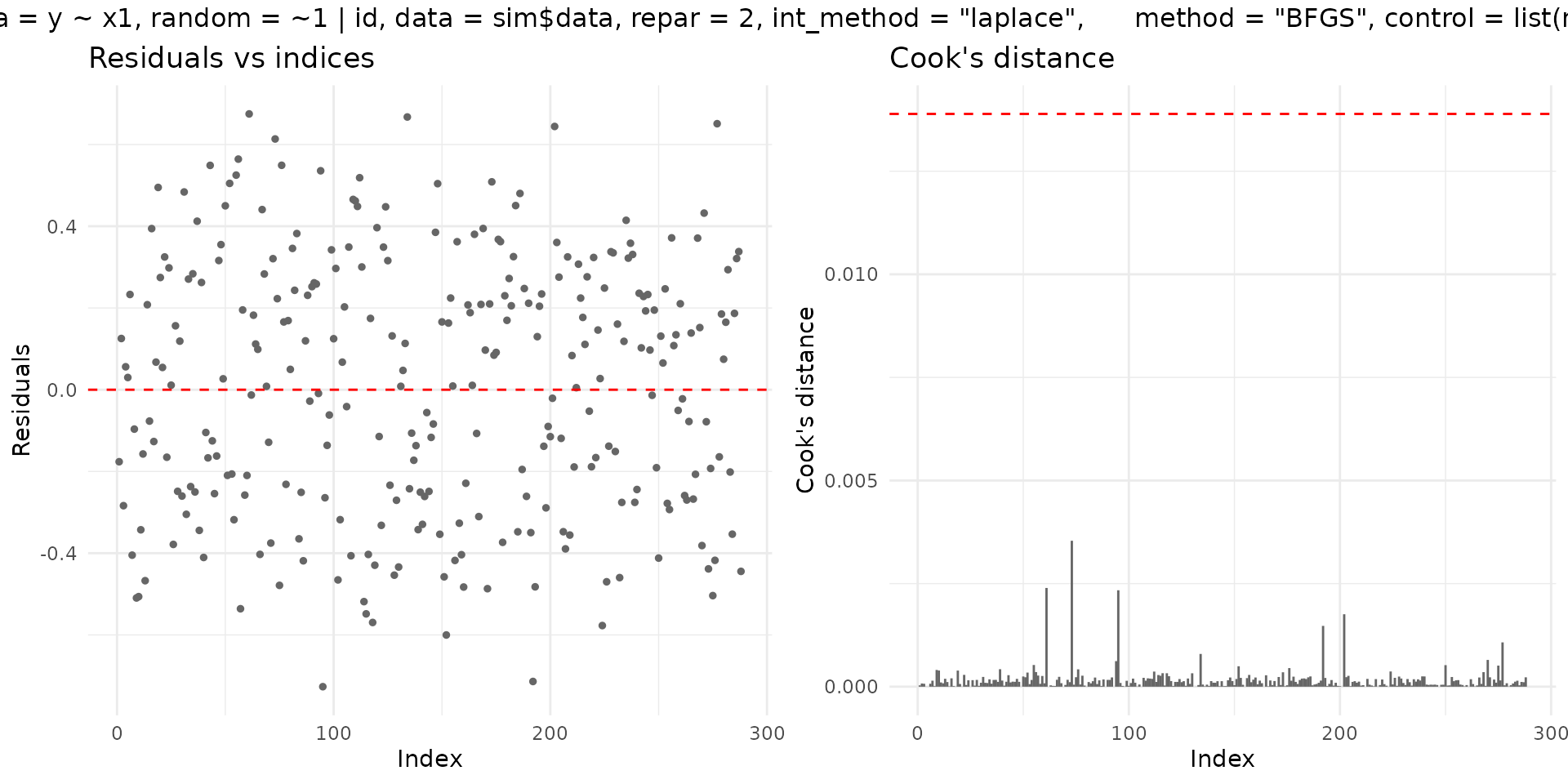
#> [1] -0.53908822  0.49503053 -0.84724816  0.16994500  0.08784679  0.73370665

Diagnostic plotting methods

plot.brsmm() supports base and ggplot2 backends:

plot(fit_mm, which = 1:4, type = "pearson")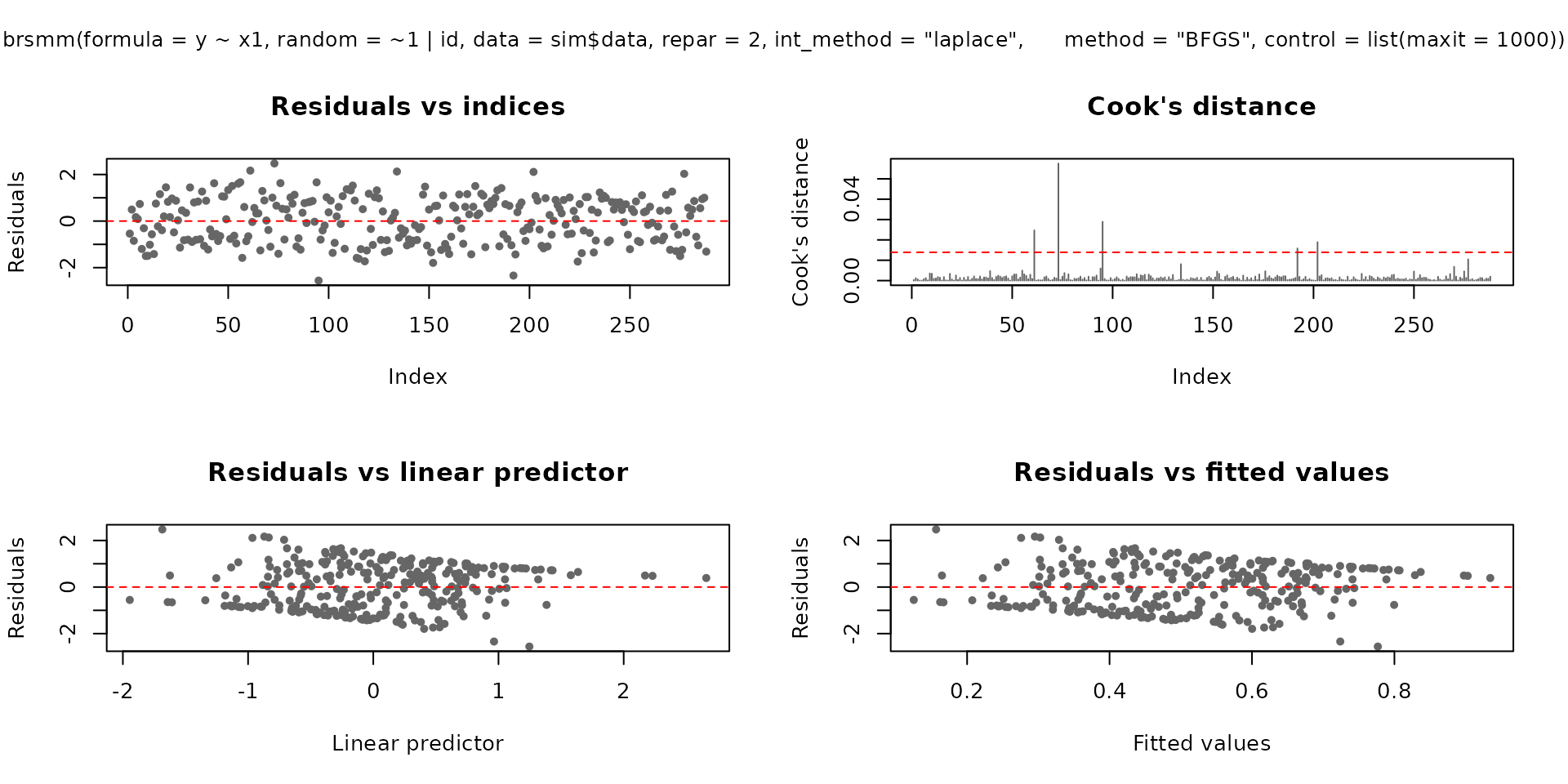


if (requireNamespace("ggplot2", quietly = TRUE)) {
  plot(fit_mm, which = 1:2, gg = TRUE)
}

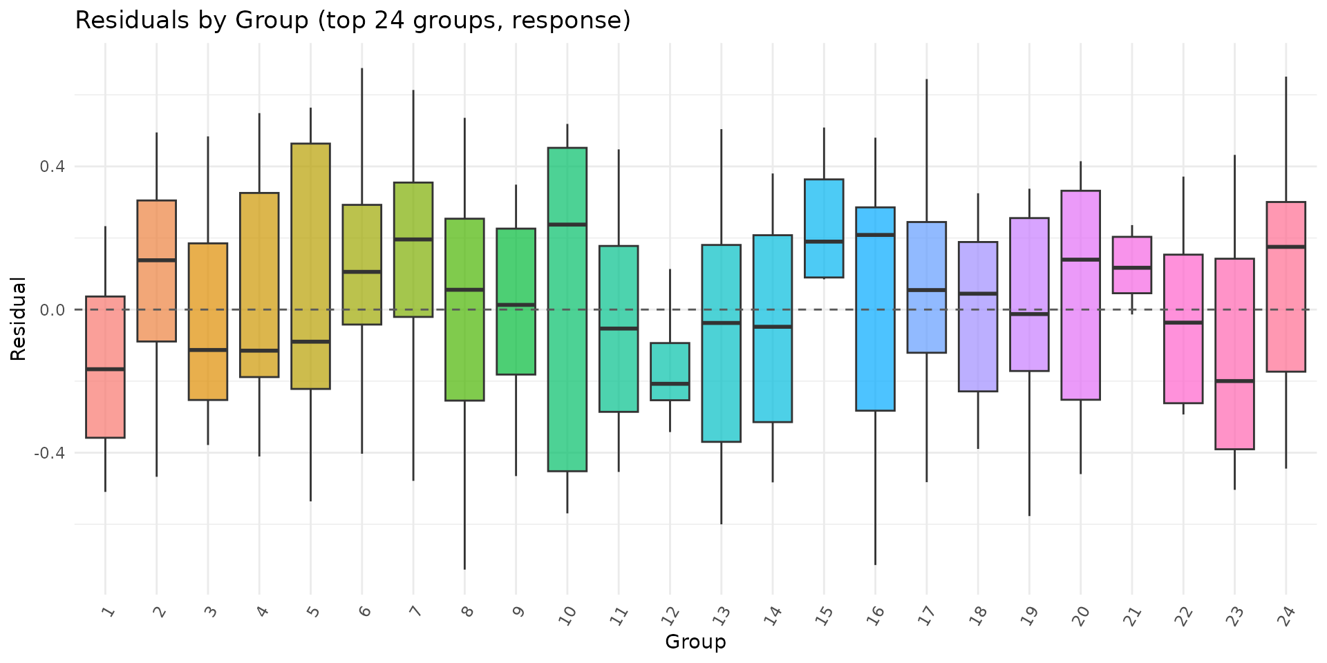
autoplot.brsmm() provides focused ggplot diagnostics:

if (requireNamespace("ggplot2", quietly = TRUE)) {
  autoplot.brsmm(fit_mm, type = "calibration")
  autoplot.brsmm(fit_mm, type = "score_dist")
  autoplot.brsmm(fit_mm, type = "ranef_qq")
  autoplot.brsmm(fit_mm, type = "residuals_by_group")
}

Prediction with `newdata`

If newdata contains unseen groups, predict.brsmm() uses random effect equal to zero for those levels.

nd <- sim$data[1:8, c("x1", "id")]
predict(fit_mm, newdata = nd, type = "response")
#> [1] 0.3562286 0.1646701 0.4037733 0.3738710 0.5300708 0.3169583 0.4348323
#> [8] 0.3063863

nd_unseen <- nd
nd_unseen$id <- factor(rep("new_cluster", nrow(nd_unseen)))
predict(fit_mm, newdata = nd_unseen, type = "response")
#> [1] 0.4449724 0.2221609 0.4952496 0.4638431 0.6203876 0.4020284 0.5271241
#> [8] 0.3902401

Statistical tests and validation workflow

Wald tests (from `summary`)

summary.brsmm() reports Wald $z$ -tests for each parameter: $z_k = \hat\theta_k / \mathrm{SE}(\hat\theta_k).$

summary(fit_mm)$coefficients
#>                      Estimate Std. Error    z value     Pr(>|z|)
#> (Intercept)        0.01051336 0.05997713  0.1752895 8.608522e-01
#> x1                 0.62964563 0.08649567  7.2795044 3.350653e-13
#> (phi)_(Intercept) -0.13626654 0.07704204 -1.7687296 7.693901e-02
#> (sd)_id           -0.84336505 0.26045257 -3.2380753 1.203390e-03

Likelihood-ratio test for nested fixed effects

For nested models with the same random-effect structure, an LR test can be computed as: $LR = 2\{\ell(\hat\theta_1)-\ell(\hat\theta_0)\},$ using a $\chi^2$ reference with parameter-count difference.

fit_null <- brsmm(
  y ~ 1,
  random = ~ 1 | id,
  data = sim$data,
  repar = 2,
  int_method = "laplace",
  method = "BFGS",
  control = list(maxit = 1000)
)

ll0 <- logLik(fit_null)
ll1 <- logLik(fit_mm)
lr_stat <- 2 * (as.numeric(ll1) - as.numeric(ll0))
df_diff <- attr(ll1, "df") - attr(ll0, "df")
p_value <- stats::pchisq(lr_stat, df = df_diff, lower.tail = FALSE)

c(LR = lr_stat, df = df_diff, p_value = p_value)

Residual diagnostics (quick checks)

r <- residuals(fit_mm, type = "pearson")
c(
  mean = mean(r),
  sd = stats::sd(r),
  q025 = as.numeric(stats::quantile(r, 0.025)),
  q975 = as.numeric(stats::quantile(r, 0.975))
)
#>        mean          sd        q025        q975 
#>  0.03803694  0.96104685 -1.56673066  1.62863050

Parameter recovery experiment

A single-fit recovery table can be produced directly from the previous fit:

est <- c(
  beta0 = coef(fit_mm, model = "mean")[1],
  beta1 = coef(fit_mm, model = "mean")[2],
  sigma_b = exp(coef(fit_mm, model = "random"))
)

true <- c(
  beta0 = sim$truth$beta[1],
  beta1 = sim$truth$beta[2],
  sigma_b = sim$truth$sigma_b
)

recovery_table <- data.frame(
  parameter = names(true),
  true = as.numeric(true),
  estimate = as.numeric(est[names(true)]),
  bias = as.numeric(est[names(true)] - true)
)
recovery_table
#>   parameter true estimate bias
#> 1     beta0 0.20       NA   NA
#> 2     beta1 0.65       NA   NA
#> 3   sigma_b 0.55       NA   NA

For a Monte Carlo recovery study, repeat simulation and fitting across replicates:

mc_recovery <- function(R = 50L, seed = 7001L) {
  set.seed(seed)
  out <- vector("list", R)

  for (r in seq_len(R)) {
    sim_r <- sim_brsmm_data(seed = seed + r)
    fit_r <- brsmm(
      y ~ x1,
      random = ~ 1 | id,
      data = sim_r$data,
      repar = 2,
      int_method = "laplace",
      method = "BFGS",
      control = list(maxit = 1000)
    )

    out[[r]] <- c(
      beta0 = coef(fit_r, model = "mean")[1],
      beta1 = coef(fit_r, model = "mean")[2],
      sigma_b = exp(coef(fit_r, model = "random"))
    )
  }

  est <- do.call(rbind, out)
  truth <- c(beta0 = 0.20, beta1 = 0.65, sigma_b = 0.55)

  data.frame(
    parameter = colnames(est),
    truth = as.numeric(truth[colnames(est)]),
    mean_est = colMeans(est),
    bias = colMeans(est) - truth[colnames(est)],
    rmse = sqrt(colMeans((sweep(est, 2, truth[colnames(est)], "-"))^2))
  )
}

mc_recovery(R = 50)

How this maps to automated package tests

The package test suite includes dedicated brsmm tests for:

fitting with Laplace integration;
one- and two-part formulas;
S3 methods (coef, vcov, summary, predict, residuals, ranef);
parameter recovery under known DGP settings.

Run locally:

devtools::test(filter = "brsmm")

References

Ferrari, S. L. P. and Cribari-Neto, F. (2004). Beta regression for modelling rates and proportions. Journal of Applied Statistics, 31(7), 799-815.

Lopes, J. E. (2024). Beta Regression for Interval-Censored Scale-Derived Outcomes. MSc Dissertation, PPGMNE/UFPR.

Pinheiro, J. C. and Bates, D. M. (2000). Mixed-Effects Models in S and S-PLUS. Springer.