Analyst Tools for betaregscale • betaregscale

Overview

This vignette presents analyst-oriented tools added to betaregscale for post-estimation workflows:

brs_table(): model comparison tables.
brs_marginaleffects(): average marginal effects (AME).
brs_predict_scoreprob(): probabilities on the original score scale.
autoplot.brs(): ggplot2 diagnostics.
brs_cv(): repeated k-fold cross-validation.

The examples use bounded scale data under the interval-censored beta regression framework of Lopes (2024).

library(betaregscale)

Mathematical foundations

Complete likelihood by censoring type

For each observation $i$ , let $\delta_i \in \{0,1,2,3\}$ indicate exact, left-censored, right-censored, or interval-censored status. With beta CDF $F(\cdot)$ , beta density $f(\cdot)$ , and interval endpoints $[l_i, u_i]$ , the contribution is:

$L_i(\theta)= \begin{cases} f(y_i; a_i, b_i), & \delta_i = 0,\\ F(u_i; a_i, b_i), & \delta_i = 1,\\ 1 - F(l_i; a_i, b_i), & \delta_i = 2,\\ F(u_i; a_i, b_i)-F(l_i; a_i, b_i), & \delta_i = 3. \end{cases}$

This is the basis for fitting, prediction, and validation metrics.

Model-comparison metrics

brs_table() reports:

$\log L(\hat\theta)$ ,
$AIC = -2\log L(\hat\theta) + 2k$ ,
$BIC = -2\log L(\hat\theta) + k\log n$ ,

where $k$ is the number of estimated parameters and $n$ is sample size.

Average marginal effects (AME)

brs_marginaleffects() computes AME by finite differences:

$\mathrm{AME}_j = \frac{1}{n}\sum_{i=1}^n \frac{\hat g_i(x_{ij}+h)-\hat g_i(x_{ij})}{h},$

with $\hat g_i$ on the requested prediction scale (response or link). For binary covariates $x_j \in \{0,1\}$ , it uses the discrete contrast $\hat g(x_j=1)-\hat g(x_j=0)$ .

Score-scale probabilities

For integer scores $s \in \{0,\dots,K\}$ , brs_predict_scoreprob() computes:

$P(Y=s)= \begin{cases} F(\mathrm{lim}/K), & s=0,\\ 1-F((K-\mathrm{lim})/K), & s=K,\\ F((s+\mathrm{lim})/K)-F((s-\mathrm{lim})/K), & 1 \le s \le K-1. \end{cases}$

These probabilities are directly aligned with interval geometry on the original instrument scale.

Cross-validation log score

In brs_cv(), fold-level predictive quality includes:

$\mathrm{log\_score} = \frac{1}{n_{test}}\sum_{i \in test}\log(p_i),$

where $p_i$ is the predictive contribution from the same censoring-rule piecewise definition shown above.

It also reports:

$\mathrm{RMSE}_{yt} = \sqrt{\frac{1}{n_{test}}\sum (y_{t,i}-\hat\mu_i)^2}, \qquad \mathrm{MAE}_{yt} = \frac{1}{n_{test}}\sum |y_{t,i}-\hat\mu_i|.$

Reproducible workflow

1) Simulate data and fit candidate models

set.seed(2026)
n <- 220
d <- data.frame(
  x1 = rnorm(n),
  x2 = rnorm(n),
  z1 = rnorm(n)
)

sim <- brs_sim(
  formula = ~ x1 + x2 | z1,
  data = d,
  beta = c(0.20, -0.45, 0.25),
  zeta = c(0.15, -0.30),
  ncuts = 100,
  repar = 2
)

fit_fixed <- brs(y ~ x1 + x2, data = sim, repar = 2)
fit_var <- brs(y ~ x1 + x2 | z1, data = sim, repar = 2)

2) Compare models in one table

tab <- brs_table(
  fixed = fit_fixed,
  variable = fit_var,
  sort_by = "AIC"
)
tab
#>      model nobs npar    logLik      AIC      BIC pseudo_r2 exact left right
#> 1 variable  220    5 -931.8646 1873.729 1890.697    0.1381     0    8    22
#> 2    fixed  220    4 -939.3243 1886.649 1900.223    0.1381     0    8    22
#>   interval prop_exact prop_left prop_right prop_interval
#> 1      190          0    0.0364        0.1        0.8636
#> 2      190          0    0.0364        0.1        0.8636

3) Estimate average marginal effects

me_mean <- brs_marginaleffects(
  fit_var,
  model = "mean",
  type = "response",
  interval = TRUE,
  n_sim = 120
)
me_mean
#>   variable         ame  std.error    ci.lower    ci.upper model     type   n
#> 1       x1 -0.10350449 0.01859635 -0.13287991 -0.06613533  mean response 220
#> 2       x2  0.07342329 0.01729846  0.04748093  0.10839857  mean response 220

me_precision <- brs_marginaleffects(
  fit_var,
  model = "precision",
  type = "link",
  interval = FALSE
)
me_precision
#>   variable        ame std.error ci.lower ci.upper     model type   n
#> 1       z1 -0.3360715        NA       NA       NA precision link 220

4) Predict score probabilities

P <- brs_predict_scoreprob(fit_var, scores = 0:10)
dim(P)
#> [1] 220  11
head(P[, 1:5])
#>          score_0     score_1     score_2     score_3     score_4
#> [1,] 0.014623303 0.017790410 0.014558715 0.013036068 0.012076830
#> [2,] 0.021451858 0.022805666 0.017769488 0.015484433 0.014073831
#> [3,] 0.046547692 0.031830606 0.021590702 0.017455271 0.015064658
#> [4,] 0.073078453 0.037104253 0.023313719 0.018090062 0.015175980
#> [5,] 0.007646182 0.010508656 0.009021869 0.008303000 0.007845942
#> [6,] 0.005023701 0.005045276 0.003869686 0.003351163 0.003037766
summary(rowSums(P))
#>     Min.  1st Qu.   Median     Mean  3rd Qu.     Max. 
#> 0.009836 0.077558 0.133484 0.150893 0.212978 0.526155

rowSums(P) should be close to 1 (up to numerical tolerance and score subset selection).

5) ggplot2 diagnostics

autoplot.brs(fit_var, type = "calibration")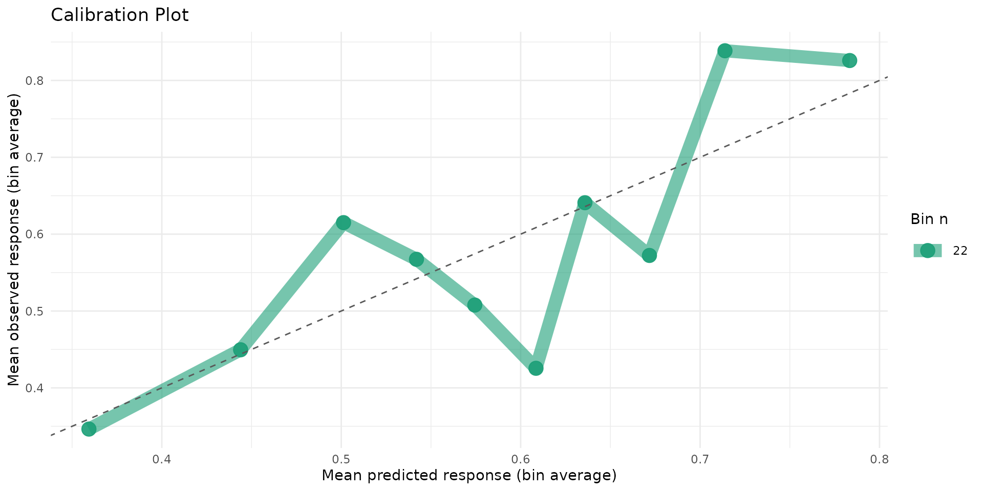

autoplot.brs(fit_var, type = "score_dist", scores = 0:20)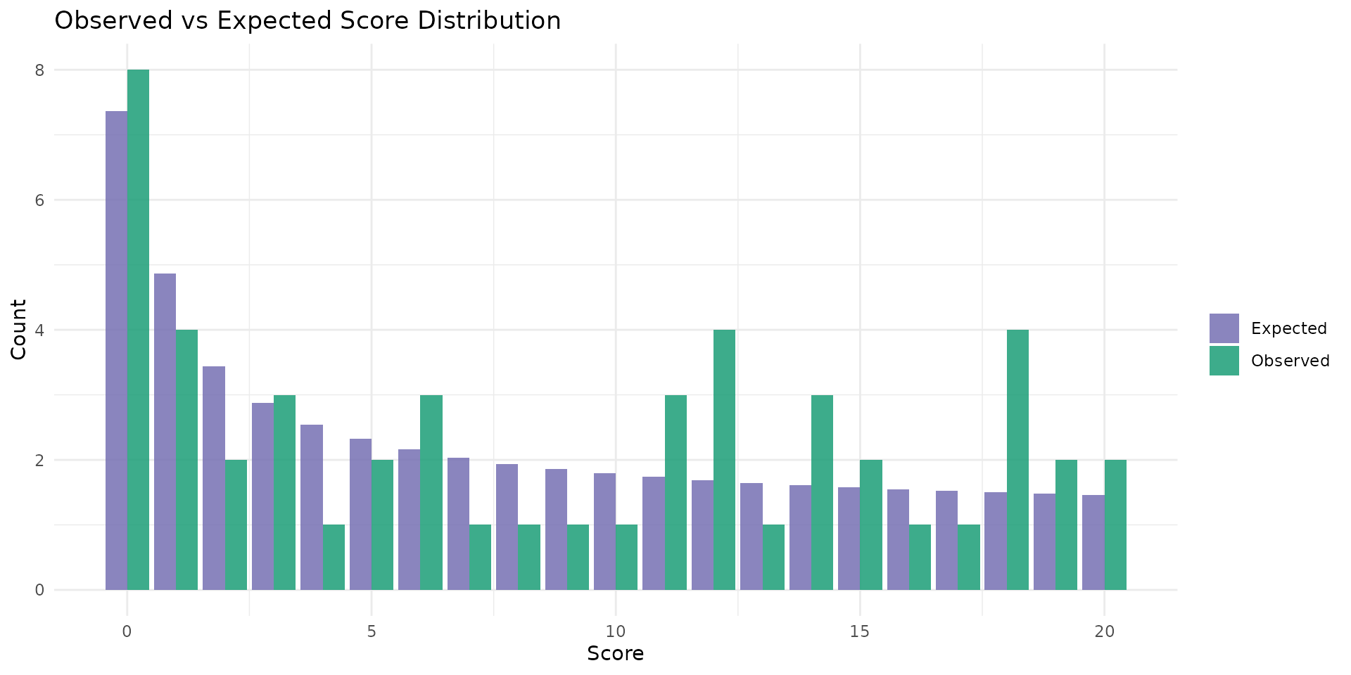

autoplot.brs(fit_var, type = "cdf", max_curves = 4)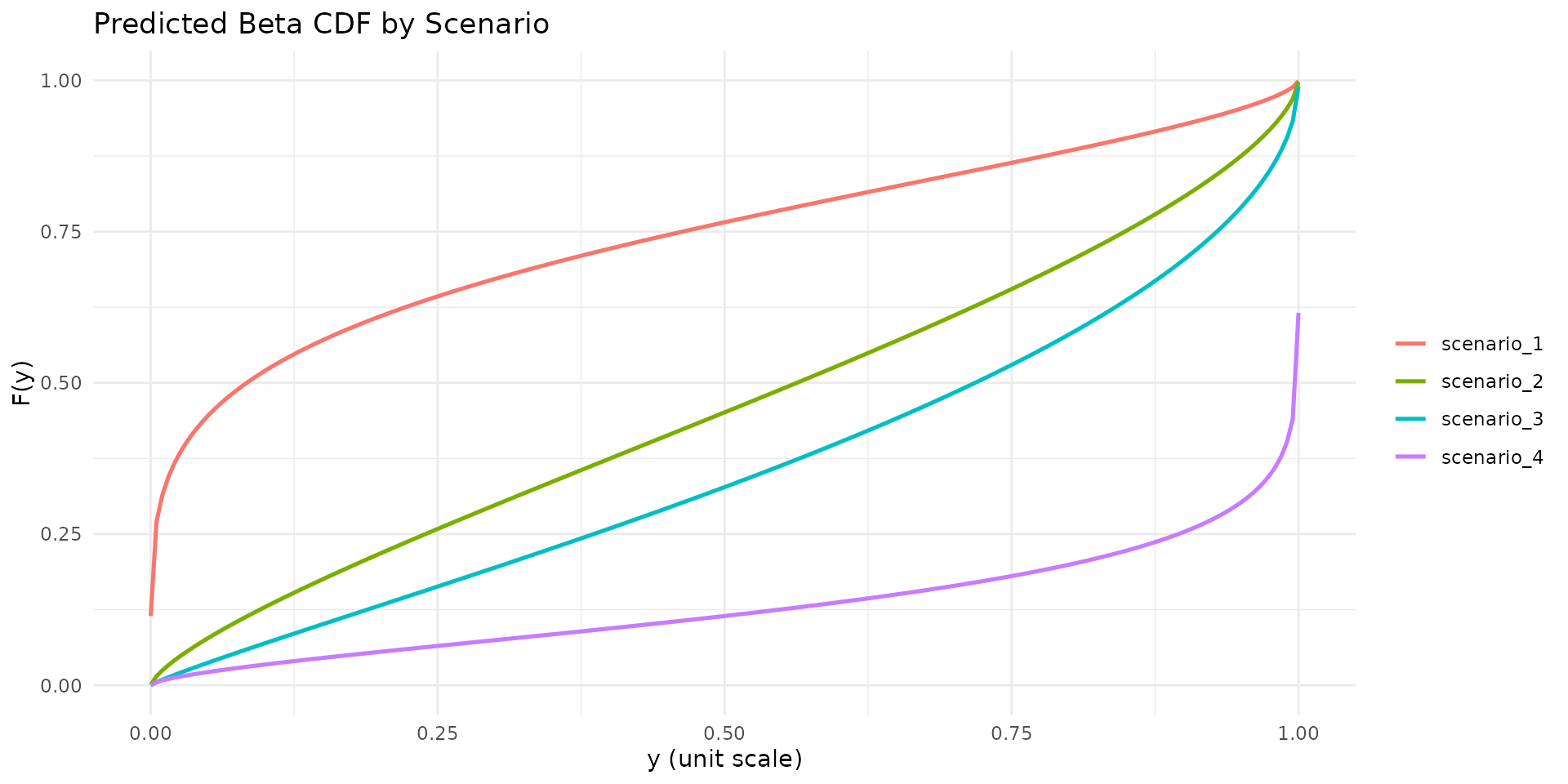

autoplot.brs(fit_var, type = "residuals_by_delta", residual_type = "rqr")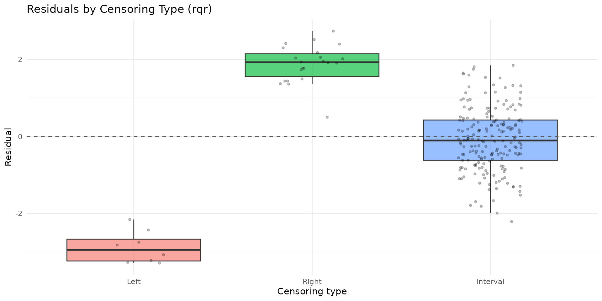

6) Repeated k-fold cross-validation

cv_res <- brs_cv(
  y ~ x1 + x2 | z1,
  data = sim,
  k = 3,
  repeats = 1,
  repar = 2,
  seed = 2026
)

cv_res
#>   repeat fold n_train n_test log_score   rmse_yt    mae_yt converged error
#> 1      1    1     146     74 -4.307714 0.3214558 0.2861862      TRUE  <NA>
#> 2      1    2     147     73 -4.317109 0.3448886 0.3031531      TRUE  <NA>
#> 3      1    3     147     73 -4.167553 0.3454093 0.3021977      TRUE  <NA>
colMeans(cv_res[, c("log_score", "rmse_yt", "mae_yt")], na.rm = TRUE)
#>  log_score    rmse_yt     mae_yt 
#> -4.2641252  0.3372512  0.2971790

Practical interpretation

Prefer the model with lower AIC/BIC and better predictive log_score.
Use AME on the response scale to communicate expected change in mean score (on the unit interval) from small covariate shifts.
Use score probabilities to translate model outputs back to clinically interpretable scale categories.
Inspect calibration and residual-by-censoring plots before inference.

References

Lopes, J. E. (2024). Beta Regression for Interval-Censored Scale-Derived Outcomes. MSc Dissertation, PPGMNE/UFPR.
Ferrari, S. and Cribari-Neto, F. (2004). Beta regression for modelling rates and proportions. Journal of Applied Statistics, 31(7), 799-815.
Hawker, G. A., Mian, S., Kendzerska, T., and French, M. (2011). Measures of adult pain: VAS, NRS, MPQ, SF-MPQ, CPGS, SF-36 BPS, and ICOAP. Arthritis Care and Research, 63(S11), S240-S252.
Hjermstad, M. J., Fayers, P. M., Haugen, D. F., et al. (2011). Comparing NRS, VRS, and VAS pain scales in adults: a systematic review. Journal of Pain and Symptom Management, 41(6), 1073-1093.