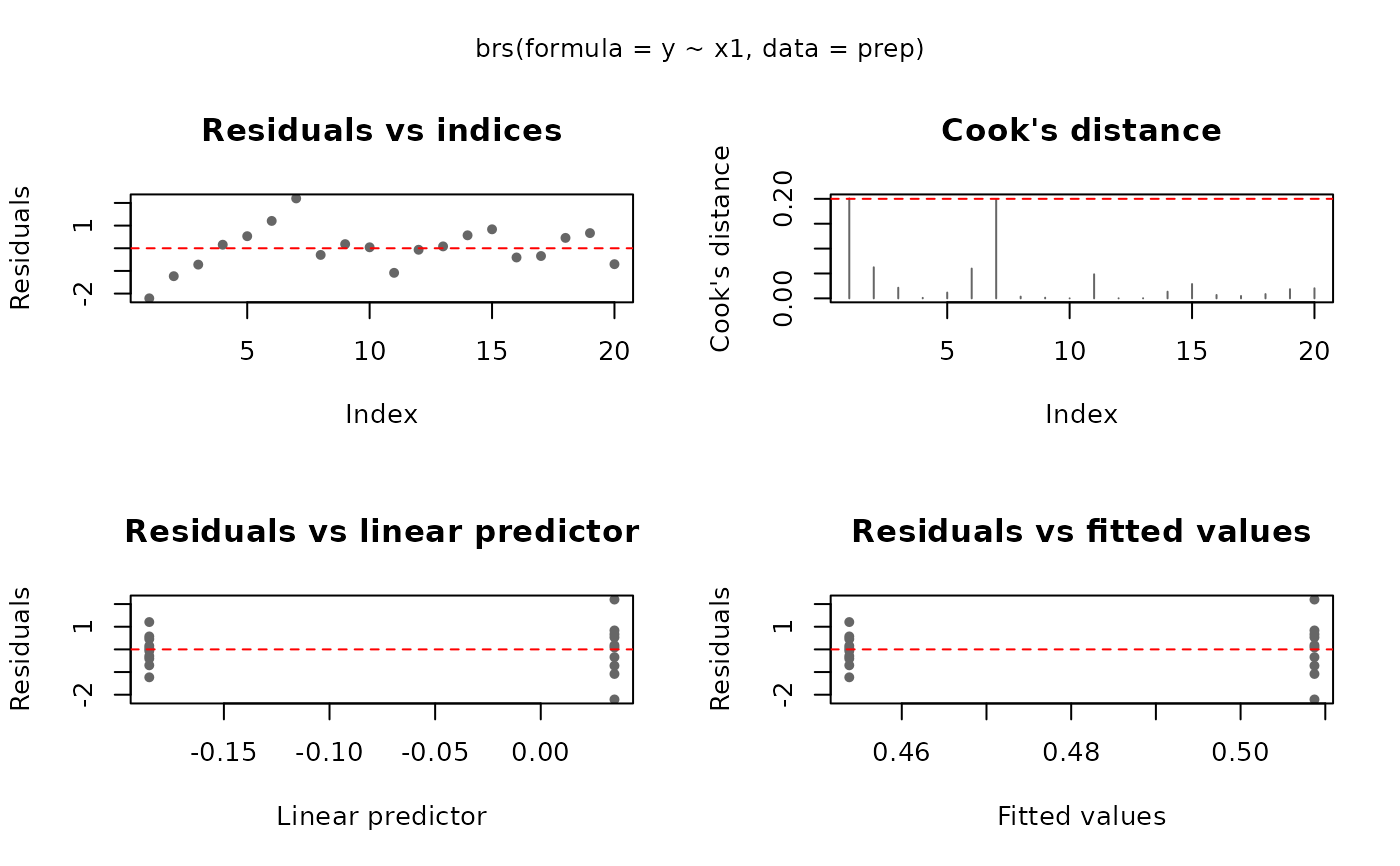
Produces up to six diagnostic plots for a fitted
"brs" model: residuals vs indices, Cook's
distance, residuals vs linear predictor, residuals vs fitted
values, a half-normal plot with simulated envelope, and
predicted vs observed.
Usage
# S3 method for class 'brs'
plot(
  x,
  which = 1:4,
  type = "rqr",
  nsim = 100L,
  level = 0.9,
  caption = c("Residuals vs indices", "Cook's distance", "Residuals vs linear predictor",
    "Residuals vs fitted values", "Half-normal plot", "Predicted vs observed"),
  sub.caption = NULL,
  ask = prod(par("mfcol")) < length(which) && dev.interactive(),
  gg = FALSE,
  title = NULL,
  theme = NULL,
  ...
)
Arguments
- x
A fitted
"brs"object.- which
Integer vector selecting which plots to draw (default
1:4).- type
Character: residual type passed to
residuals.brs(default"rqr").- nsim
Integer: number of simulations for the half-normal envelope (default 100).
- level
Numeric: confidence level for the envelope (default 0.9).
- caption
Character vector of panel captions.
- sub.caption
Subtitle; defaults to the model call.
- ask
Logical: prompt before each page of plots?
- gg
Logical: use ggplot2? (default
FALSE).- title
Optional global title for ggplot output. If
NULL, panel captions are used.- theme
Optional ggplot2 theme object (e.g.,
ggplot2::theme_bw()). IfNULL, a minimal theme is used.- ...
Further arguments passed to base
plot().
Examples
# \donttest{
dat <- data.frame(
  y = c(
    0, 5, 20, 50, 75, 90, 100, 30, 60, 45,
    10, 40, 55, 70, 85, 25, 35, 65, 80, 15
  ),
  x1 = rep(c(1, 2), 10)
)
prep <- brs_prep(dat, ncuts = 100)
#> brs_prep: n = 20 | exact = 0, left = 1, right = 1, interval = 18
fit <- brs(y ~ x1, data = prep)
plot(fit, which = 1:4)

# }
# }