Fits regression models using the Generalized Kumaraswamy (GKw) family of distributions for modeling response variables strictly bounded in the interval (0, 1). The function provides a unified interface for fitting seven nested submodels of the GKw family, allowing flexible modeling of proportions, rates, and other bounded continuous outcomes through regression on distributional parameters.
Maximum Likelihood Estimation is performed via automatic differentiation using
the TMB (Template Model Builder) package, ensuring computational efficiency and
numerical accuracy. The interface follows standard R regression modeling
conventions similar to lm, glm, and
betareg, making it immediately familiar to R users.
Usage
gkwreg(
  formula,
  data,
  family = c("gkw", "bkw", "kkw", "ekw", "mc", "kw", "beta"),
  link = NULL,
  link_scale = NULL,
  subset = NULL,
  weights = NULL,
  offset = NULL,
  na.action = getOption("na.action"),
  contrasts = NULL,
  control = gkw_control(),
  model = TRUE,
  x = FALSE,
  y = TRUE,
  ...
)
Arguments
- formula
An object of class
Formula(or one that can be coerced to that class). The formula uses extended syntax to specify potentially different linear predictors for each distribution parameter:y ~ model_alpha | model_beta | model_gamma | model_delta | model_lambdawhere:
yis the response variable (must be in the open interval (0, 1))model_alphaspecifies predictors for the \(\alpha\) parametermodel_betaspecifies predictors for the \(\beta\) parametermodel_gammaspecifies predictors for the \(\gamma\) parametermodel_deltaspecifies predictors for the \(\delta\) parametermodel_lambdaspecifies predictors for the \(\lambda\) parameter
If a part is omitted or specified as
~ 1, an intercept-only model is used for that parameter. Parts corresponding to fixed parameters (determined byfamily) are automatically ignored. See Details and Examples for proper usage.- data
A data frame containing the variables specified in
formula. Standard R subsetting and missing value handling apply.- family
A character string specifying the distribution family from the Generalized Kumaraswamy hierarchy. Must be one of:
"gkw"Generalized Kumaraswamy (default). Five parameters: \(\alpha, \beta, \gamma, \delta, \lambda\). Most flexible, suitable when data show complex behavior not captured by simpler families.
"bkw"Beta-Kumaraswamy. Four parameters: \(\alpha, \beta, \gamma, \delta\) (fixes \(\lambda = 1\)). Combines Beta and Kumaraswamy flexibility.
"kkw"Kumaraswamy-Kumaraswamy. Four parameters: \(\alpha, \beta, \delta, \lambda\) (fixes \(\gamma = 1\)). Alternative four-parameter generalization.
"ekw"Exponentiated Kumaraswamy. Three parameters: \(\alpha, \beta, \lambda\) (fixes \(\gamma = 1, \delta = 0\)). Adds flexibility to standard Kumaraswamy.
"mc"McDonald (Beta Power). Three parameters: \(\gamma, \delta, \lambda\) (fixes \(\alpha = 1, \beta = 1\)). Generalization of Beta distribution.
"kw"Kumaraswamy. Two parameters: \(\alpha, \beta\) (fixes \(\gamma = 1, \delta = 0, \lambda = 1\)). Computationally efficient alternative to Beta with closed-form CDF.
"beta"Beta distribution. Two parameters: \(\gamma, \delta\) (fixes \(\alpha = 1, \beta = 1, \lambda = 1\)). Standard choice for proportions and rates, corresponds to shape1 = \(\gamma\), shape2 = \(\delta\).
See Details for guidance on family selection.
- link
Link function(s) for the distributional parameters. Can be specified as:
Single character string: Same link for all relevant parameters. Example:
link = "log"applies log link to all parameters.Named list: Parameter-specific links for fine control. Example:
link = list(alpha = "log", beta = "log", delta = "logit")
Default links (used if
link = NULL):"log"for \(\alpha, \beta, \gamma, \lambda\) (positive parameters)"logit"for \(\delta\) (parameter in (0, 1))
Available link functions:
"log"Logarithmic link. Maps \((0, \infty) \to (-\infty, \infty)\). Ensures positivity. Most common for shape parameters.
"logit"Logistic link. Maps \((0, 1) \to (-\infty, \infty)\). Standard for probability-type parameters like \(\delta\).
"probit"Probit link using normal CDF. Maps \((0, 1) \to (-\infty, \infty)\). Alternative to logit, symmetric tails.
"cloglog"Complementary log-log. Maps \((0, 1) \to (-\infty, \infty)\). Asymmetric, useful for skewed probabilities.
"cauchy"Cauchy link using Cauchy CDF. Maps \((0, 1) \to (-\infty, \infty)\). Heavy-tailed alternative to probit.
"identity"Identity link (no transformation). Use with caution; does not guarantee parameter constraints.
"sqrt"Square root link. Maps \(x \to \sqrt{x}\). Variance-stabilizing for some contexts.
"inverse"Inverse link. Maps \(x \to 1/x\). Useful for rate-type parameters.
"inverse-square"Inverse squared link. Maps \(x \to 1/x^2\).
- link_scale
Numeric scale factor(s) controlling the transformation intensity of link functions. Can be:
Single numeric: Same scale for all parameters.
Named list: Parameter-specific scales for fine-tuning. Example:
link_scale = list(alpha = 10, beta = 10, delta = 1)
Default scales (used if
link_scale = NULL):10 for \(\alpha, \beta, \gamma, \lambda\)
1 for \(\delta\)
Larger values produce more gradual transformations; smaller values produce more extreme transformations. For probability-type links (logit, probit), smaller scales (e.g., 0.5-2) create steeper response curves, while larger scales (e.g., 5-20) create gentler curves. Adjust if convergence issues arise or if you need different response sensitivities.
- subset
Optional vector specifying a subset of observations to be used in fitting. Can be a logical vector, integer indices, or expression evaluating to one of these. Standard R subsetting rules apply.
- weights
Optional numeric vector of prior weights (e.g., frequency weights) for observations. Should be non-negative. Currently experimental; use with caution and validate results.
- offset
Optional numeric vector or matrix specifying an a priori known component to be included in the linear predictor(s). If a vector, it is applied to the first parameter's predictor. If a matrix, columns correspond to parameters in order (\(\alpha, \beta, \gamma, \delta, \lambda\)). Offsets are added to the linear predictor before applying the link function.
- na.action
A function specifying how to handle missing values (
NAs). Options include:na.failStop with error if
NAs present (default viagetOption("na.action"))na.omitRemove observations with
NAsna.excludeLike
na.omitbut preserves original length in residuals/fitted values
See
na.actionfor details.- contrasts
Optional list specifying contrasts for factor variables in the model. Format: named list where names are factor variable names and values are contrast specifications. See
contrastsand thecontrasts.argargument ofmodel.matrix.- control
A list of control parameters from
gkw_controlspecifying technical details of the fitting process. This includes:Optimization algorithm (
method)Starting values (
start)Fixed parameters (
fixed)Convergence tolerances (
maxit,reltol,abstol)Hessian computation (
hessian)Verbosity (
silent,trace)
Default is
gkw_control()which uses sensible defaults for most problems. Seegkw_controlfor complete documentation of all options. Most users never need to modify control parameters.- model
Logical. If
TRUE(default), the model frame (data frame containing all variables used in fitting) is returned as componentmodelof the result. Useful for prediction and diagnostics. Set toFALSEto reduce object size.- x
Logical. If
TRUE, the list of model matrices (one for each modeled parameter) is returned as componentx. DefaultFALSE. Set toTRUEif you need direct access to design matrices for custom calculations.- y
Logical. If
TRUE(default), the response vector (after processing byna.actionandsubset) is returned as componenty. Useful for residual calculations and diagnostics.- ...
Additional arguments. Currently used only for backward compatibility with deprecated arguments from earlier versions. Using deprecated arguments triggers informative warnings with migration guidance. Examples of deprecated arguments:
plot,conf.level,method,start,fixed,hessian,silent,optimizer.control. These should now be passed via thecontrolargument.
Value
An object of class "gkwreg", which is a list containing the following
components. Standard S3 methods are available for this class (see Methods section).
Model Specification:
callThe matched function call
formulaThe
Formulaobject usedfamilyCharacter string: distribution family used
linkNamed list: link functions for each parameter
link_scaleNamed list: link scale values for each parameter
param_namesCharacter vector: names of parameters for this family
fixed_paramsNamed list: parameters fixed by family definition
controlThe
gkw_controlobject used for fitting
Parameter Estimates:
coefficientsNamed numeric vector: estimated regression coefficients (on link scale). Names follow the pattern "parameter:predictor", e.g., "alpha:(Intercept)", "alpha:x1", "beta:(Intercept)", "beta:x2".
fitted_parametersNamed list: mean values for each distribution parameter (\(\alpha, \beta, \gamma, \delta, \lambda\)) averaged across all observations
parameter_vectorsNamed list: observation-specific parameter values. Contains vectors
alphaVec,betaVec,gammaVec,deltaVec,lambdaVec, each of lengthnobs
Fitted Values and Residuals:
fitted.valuesNumeric vector: fitted mean values \(E[Y|X]\) for each observation
residualsNumeric vector: response residuals (observed - fitted) for each observation
Inference:
vcovVariance-covariance matrix of coefficient estimates. Only present if
control$hessian = TRUE.NULLotherwise.seNumeric vector: standard errors of coefficients. Only present if
control$hessian = TRUE.NULLotherwise.
Model Fit Statistics:
loglikNumeric: maximized log-likelihood value
aicNumeric: Akaike Information Criterion (AIC = -2loglik + 2npar)
bicNumeric: Bayesian Information Criterion (BIC = -2*loglik + log(nobs)*npar)
devianceNumeric: deviance (-2 * loglik)
df.residualInteger: residual degrees of freedom (nobs - npar)
nobsInteger: number of observations used in fit
nparInteger: total number of estimated parameters
Diagnostic Statistics:
rmseNumeric: Root Mean Squared Error of response residuals
efron_r2Numeric: Efron's pseudo R-squared (1 - SSE/SST, where SSE = sum of squared errors, SST = total sum of squares)
mean_absolute_errorNumeric: Mean Absolute Error of response residuals
Optimization Details:
convergenceLogical:
TRUEif optimizer converged successfully,FALSEotherwisemessageCharacter: convergence message from optimizer
iterationsInteger: number of iterations used by optimizer
methodCharacter: optimization method used (e.g., "nlminb", "BFGS")
Optional Components (returned if requested via model, x, y):
modelData frame: the model frame (if
model = TRUE)xNamed list: model matrices for each parameter (if
x = TRUE)yNumeric vector: the response variable (if
y = TRUE)
Internal:
tmb_objectThe raw object returned by
MakeADFun. Contains the TMB automatic differentiation function and environment. Primarily for internal use and advanced debugging.
Details
Distribution Family Selection
The Generalized Kumaraswamy family provides a flexible hierarchy for modeling bounded responses. Selection should be guided by:
1. Start Simple: Begin with two-parameter families ("kw" or
"beta") unless you have strong reasons to use more complex models.
2. Model Comparison: Use information criteria (AIC, BIC) and likelihood ratio tests to compare nested models:
  # Fit sequence of nested models
  fit_kw   <- gkwreg(y ~ x, data, family = "kw")
  fit_ekw  <- gkwreg(y ~ x, data, family = "ekw")
  fit_gkw  <- gkwreg(y ~ x, data, family = "gkw")

  # Compare via AIC
  AIC(fit_kw, fit_ekw, fit_gkw)

  # Formal test (nested models only)
  anova(fit_kw, fit_ekw, fit_gkw)
3. Family Characteristics:
Beta: Traditional choice, well-understood, good for symmetric or moderately skewed data
Kumaraswamy (kw): Computationally efficient alternative to Beta, closed-form CDF, similar flexibility
Exponentiated Kumaraswamy (ekw): Adds flexibility for extreme values and heavy tails
Beta-Kumaraswamy (bkw), Kumaraswamy-Kumaraswamy (kkw): Four-parameter alternatives when three parameters insufficient
McDonald (mc): Beta generalization via power parameter, useful for J-shaped distributions
Kumaraswamy-Kumaraswamy (kkw): Most flexible, use only when simpler families inadequate. It extends kw
Generalized Kumaraswamy (gkw): Most flexible, use only when simpler families inadequate
4. Avoid Overfitting: More different parameters better model. Use cross-validation or hold-out validation to assess predictive performance.
Formula Specification
The extended formula syntax allows different predictors for each parameter:
Basic Examples:
  # Same predictors for both parameters (two-parameter family)
  y ~ x1 + x2
  # Equivalent to: y ~ x1 + x2 | x1 + x2

  # Different predictors per parameter
  y ~ x1 + x2 | x3 + x4
  # alpha depends on x1, x2
  # beta depends on x3, x4

  # Intercept-only for some parameters
  y ~ x1 | 1
  # alpha depends on x1
  # beta has only intercept

  # Complex specification (five-parameter family)
  y ~ x1 | x2 | x3 | x4 | x5
  # alpha ~ x1, beta ~ x2, gamma ~ x3, delta ~ x4, lambda ~ x5
Important Notes:
Formula parts correspond to parameters in order: \(\alpha\), \(\beta\), \(\gamma\), \(\delta\), \(\lambda\)
Unused parts (due to family constraints) are automatically ignored
Use
.to include all predictors:y ~ . | .Standard R formula features work: interactions (
x1:x2), polynomials (poly(x, 2)), transformations (log(x)), etc.
Link Functions and Scales
Link functions map the range of distributional parameters to the real line, ensuring parameter constraints are satisfied during optimization.
Choosing Links:
Defaults are usually best: The automatic choices (log for shape parameters, logit for delta) work well in most cases
Alternative links: Consider if you have theoretical reasons (e.g., probit for latent variable interpretation) or convergence issues
Identity link: Avoid unless you have constraints elsewhere; can lead to invalid parameter values during optimization
Link Scales:
The link_scale parameter controls transformation intensity. Think of it
as a "sensitivity" parameter:
Larger values (e.g., 20): Gentler response to predictor changes
Smaller values (e.g., 2): Steeper response to predictor changes
Default (10): Balanced, works well for most cases
Adjust only if:
Convergence difficulties arise
You need very steep or very gentle response curves
Predictors have unusual scales (very large or very small)
Optimization and Convergence
The default optimizer (method = "nlminb") works well for most problems.
If convergence issues occur:
1. Check Data:
Ensure response is strictly in (0, 1)
Check for extreme outliers or influential points
Verify predictors aren't perfectly collinear
Consider rescaling predictors to similar ranges
2. Try Alternative Optimizers:
  # BFGS often more robust for difficult problems
  fit <- gkwreg(y ~ x, data,
                control = gkw_control(method = "BFGS"))

  # Nelder-Mead for non-smooth objectives
  fit <- gkwreg(y ~ x, data,
                control = gkw_control(method = "Nelder-Mead"))
3. Adjust Tolerances:
  # Increase iterations and loosen tolerance
  fit <- gkwreg(y ~ x, data,
                control = gkw_control(maxit = 1000, reltol = 1e-6))
4. Provide Starting Values:
  # Fit simpler model first, use as starting values
  fit_simple <- gkwreg(y ~ 1, data, family = "kw")
  start_vals <- list(
    alpha = c(coef(fit_simple)[1], rep(0, ncol(X_alpha) - 1)),
    beta  = c(coef(fit_simple)[2], rep(0, ncol(X_beta) - 1))
  )
  fit_complex <- gkwreg(y ~ x1 + x2 | x3 + x4, data, family = "kw",
                         control = gkw_control(start = start_vals))
5. Simplify Model:
Use simpler family (e.g., "kw" instead of "gkw")
Reduce number of predictors
Use intercept-only for some parameters
Standard Errors and Inference
By default, standard errors are computed via the Hessian matrix at the MLE. This provides valid asymptotic standard errors under standard regularity conditions.
When Standard Errors May Be Unreliable:
Small sample sizes (n < 30-50 per parameter)
Parameters near boundaries
Highly collinear predictors
Mis-specified models
Alternatives:
Bootstrap confidence intervals (more robust, computationally expensive)
Profile likelihood intervals via
confint(..., type = "profile")(not yet implemented)Cross-validation for predictive performance assessment
To skip Hessian computation (faster, no SEs):
  fit <- gkwreg(y ~ x, data,
                control = gkw_control(hessian = FALSE))
Model Diagnostics
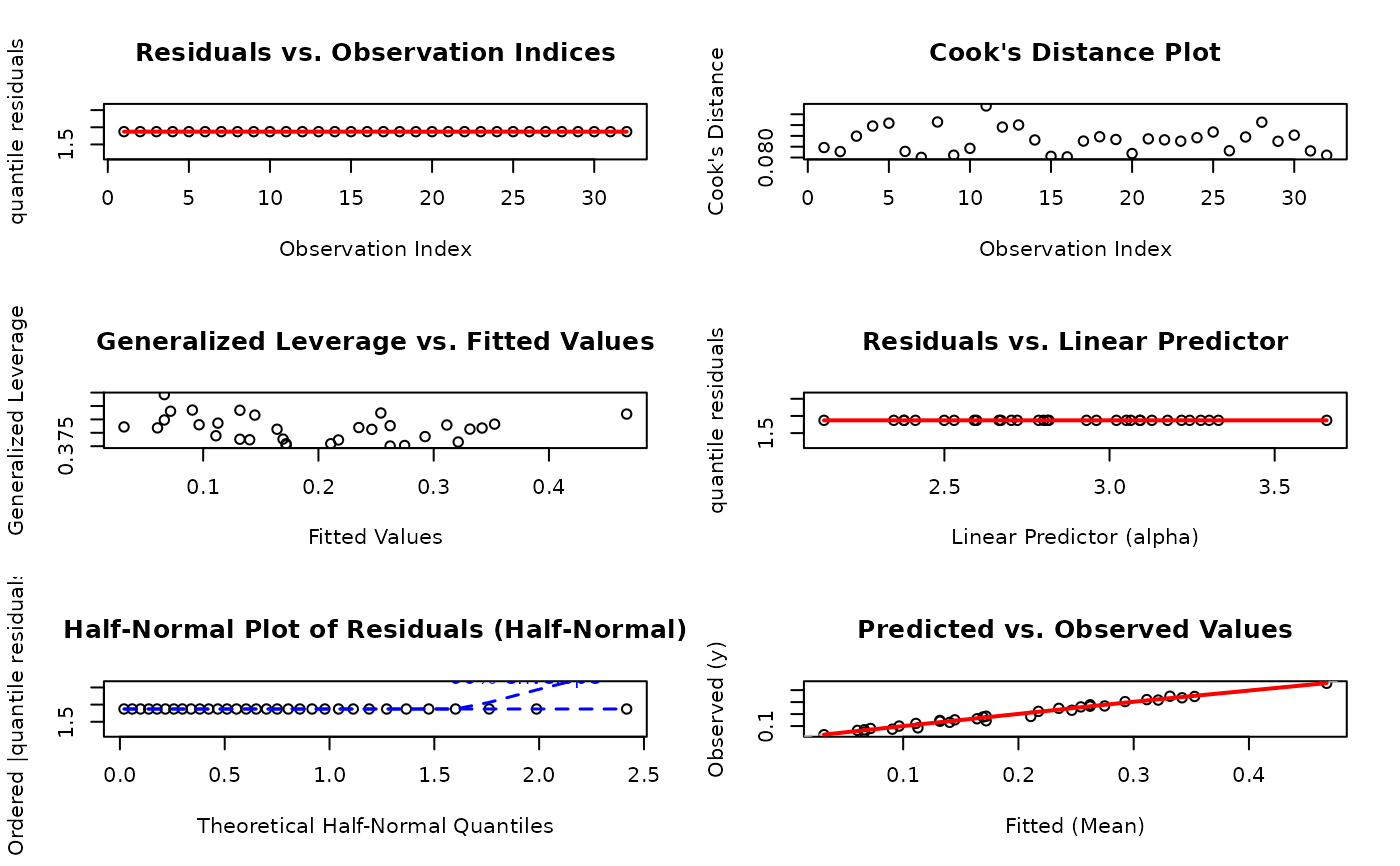
Always check model adequacy using diagnostic plots:
Key diagnostics:
Residual plots: Check for patterns, heteroscedasticity
Half-normal plot: Assess distributional adequacy
Cook's distance: Identify influential observations
Predicted vs observed: Overall fit quality
See plot.gkwreg for detailed interpretation guidance.
Computational Considerations
Performance Tips:
GKw family: Most computationally expensive (~2-5x slower than kw/beta)
Beta/Kw families: Fastest, use when adequate
Large datasets (n > 10,000): Consider sampling for exploratory analysis
TMB uses automatic differentiation: Fast gradient/Hessian computation
Disable Hessian (
hessian = FALSE) for faster fitting without SEs
Memory Usage:
Set
model = FALSE,x = FALSE,y = FALSEto reduce object size (but limits some post-fitting capabilities)Hessian matrix scales as O(p<U+00B2>) where p = number of parameters
Methods
The following S3 methods are available for objects of class "gkwreg":
Basic Methods:
print.gkwreg: Print basic model informationsummary.gkwreg: Detailed model summary with coefficient tables, tests, and fit statisticscoef.gkwreg: Extract coefficientsvcov.gkwreg: Extract variance-covariance matrixlogLik: Extract log-likelihood
Prediction and Fitted Values:
fitted.gkwreg: Extract fitted valuesresiduals.gkwreg: Extract residuals (multiple types available)predict.gkwreg: Predict on new data
Inference:
confint.gkwreg: Confidence intervals for parametersanova.gkwreg: Compare nested models via likelihood ratio tests
Diagnostics:
plot.gkwreg: Comprehensive diagnostic plots (6 types)
References
Generalized Kumaraswamy Distribution:
Cordeiro, G. M., & de Castro, M. (2011). A new family of generalized distributions. Journal of Statistical Computation and Simulation, 81(7), 883-898. doi:10.1080/00949650903530745
Kumaraswamy Distribution:
Kumaraswamy, P. (1980). A generalized probability density function for double-bounded random processes. Journal of Hydrology, 46(1-2), 79-88. doi:10.1016/0022-1694(80)90036-0
Jones, M. C. (2009). Kumaraswamy's distribution: A beta-type distribution with some tractability advantages. Statistical Methodology, 6(1), 70-81. doi:10.1016/j.stamet.2008.04.001
Beta Regression:
Ferrari, S. L. P., & Cribari-Neto, F. (2004). Beta regression for modelling rates and proportions. Journal of Applied Statistics, 31(7), 799-815. doi:10.1080/0266476042000214501
Smithson, M., & Verkuilen, J. (2006). A better lemon squeezer? Maximum-likelihood regression with beta-distributed dependent variables. Psychological Methods, 11(1), 54-71. doi:10.1037/1082-989X.11.1.54
Template Model Builder (TMB):
Kristensen, K., Nielsen, A., Berg, C. W., Skaug, H., & Bell, B. M. (2016). TMB: Automatic Differentiation and Laplace Approximation. Journal of Statistical Software, 70(5), 1-21. doi:10.18637/jss.v070.i05
Related Software:
Zeileis, A., & Croissant, Y. (2010). Extended Model Formulas in R: Multiple Parts and Multiple Responses. Journal of Statistical Software, 34(1), 1-13. doi:10.18637/jss.v034.i01
See also
Control and Inference:
gkw_control for fitting control parameters,
confint.gkwreg for confidence intervals,
anova.gkwreg for model comparison
Methods:
summary.gkwreg, plot.gkwreg,
coef.gkwreg, vcov.gkwreg,
fitted.gkwreg, residuals.gkwreg,
predict.gkwreg
Distributions:
dgkw, pgkw,
qgkw, rgkw
for the GKw distribution family functions
Related Packages:
betareg for traditional beta regression,
Formula for extended formula interface,
MakeADFun for TMB functionality
Examples
# \donttest{
# SECTION 1: Basic Usage - Getting Started
# Load packages and data
library(gkwreg)
library(gkwdist)
data(GasolineYield)
# Example 1.1: Simplest possible model (intercept-only, all defaults)
fit_basic <- gkwreg(yield ~ 1, data = GasolineYield, family = "kw")
summary(fit_basic)
#>
#> Generalized Kumaraswamy Regression Model Summary
#>
#> Family: kw
#>
#> Call:
#> gkwreg(formula = yield ~ 1, data = GasolineYield, family = "kw")
#>
#> Residuals:
#> Min Q1.25% Median Mean Q3.75% Max
#> -0.1688 -0.0803 -0.0188 -0.0002 0.0737 0.2602
#>
#> Coefficients:
#> Estimate Std. Error z value Pr(>|z|)
#> alpha:(Intercept) 0.6342 0.1538 4.124 3.73e-05 ***
#> beta:(Intercept) 2.7951 0.4319 6.472 9.68e-11 ***
#> ---
#> Signif. codes: 0 ‘***’ 0.001 ‘**’ 0.01 ‘*’ 0.05 ‘.’ 0.1 ‘ ’ 1
#>
#> Confidence intervals (95%):
#> 3% 98%
#> alpha:(Intercept) 0.3328 0.9356
#> beta:(Intercept) 1.9486 3.6416
#>
#> Link functions:
#> alpha: log
#> beta: log
#>
#> Fitted parameter means:
#> alpha: 1.886
#> beta: 16.35
#> gamma: 1
#> delta: 0
#> lambda: 1
#>
#> Model fit statistics:
#> Number of observations: 32
#> Number of parameters: 2
#> Residual degrees of freedom: 30
#> Log-likelihood: 28.51
#> AIC: -53.02
#> BIC: -50.09
#> RMSE: 0.1055
#> Efron's R2: -4.747e-06
#> Mean Absolute Error: 0.09088
#>
#> Convergence status: Successful
#> Iterations: 11
#>
# Example 1.2: Model with predictors (uses all defaults)
# Default: family = "gkw", method = "nlminb", hessian = TRUE
fit_default <- gkwreg(yield ~ batch + temp, data = GasolineYield)
#> Warning: NaNs produced
summary(fit_default)
#>
#> Generalized Kumaraswamy Regression Model Summary
#>
#> Family: gkw
#>
#> Call:
#> gkwreg(formula = yield ~ batch + temp, data = GasolineYield)
#>
#> Residuals:
#> Min Q1.25% Median Mean Q3.75% Max
#> -0.0235 -0.0071 -0.0017 -0.0002 0.0072 0.0285
#>
#> Coefficients:
#> Estimate Std. Error z value Pr(>|z|)
#> alpha:(Intercept) -1.419609 0.656437 -2.163 0.0306 *
#> alpha:batch1 0.918493 0.032363 28.381 < 2e-16 ***
#> alpha:batch2 0.676321 0.034621 19.535 < 2e-16 ***
#> alpha:batch3 0.781482 0.034584 22.596 < 2e-16 ***
#> alpha:batch4 0.557254 0.032499 17.147 < 2e-16 ***
#> alpha:batch5 0.562413 0.034496 16.304 < 2e-16 ***
#> alpha:batch6 0.539372 0.034684 15.551 < 2e-16 ***
#> alpha:batch7 0.308690 0.032490 9.501 < 2e-16 ***
#> alpha:batch8 0.254506 0.034577 7.361 1.83e-13 ***
#> alpha:batch9 0.198131 0.038558 5.138 2.77e-07 ***
#> alpha:temp 0.005403 NaN NaN NaN
#> beta:(Intercept) 5.512391 2.714173 2.031 0.0423 *
#> gamma:(Intercept) 2.559268 2.292375 1.116 0.2642
#> delta:(Intercept) -2.153376 2.502826 -0.860 0.3896
#> lambda:(Intercept) 2.191087 2.320556 0.944 0.3451
#> ---
#> Signif. codes: 0 ‘***’ 0.001 ‘**’ 0.01 ‘*’ 0.05 ‘.’ 0.1 ‘ ’ 1
#>
#> Confidence intervals (95%):
#> 3% 98%
#> alpha:(Intercept) -2.7062 -0.1330
#> alpha:batch1 0.8551 0.9819
#> alpha:batch2 0.6085 0.7442
#> alpha:batch3 0.7137 0.8493
#> alpha:batch4 0.4936 0.6210
#> alpha:batch5 0.4948 0.6300
#> alpha:batch6 0.4714 0.6074
#> alpha:batch7 0.2450 0.3724
#> alpha:batch8 0.1867 0.3223
#> alpha:batch9 0.1226 0.2737
#> alpha:temp NaN NaN
#> beta:(Intercept) 0.1927 10.8321
#> gamma:(Intercept) -1.9337 7.0522
#> delta:(Intercept) -7.0588 2.7521
#> lambda:(Intercept) -2.3571 6.7393
#>
#> Link functions:
#> alpha: log
#> beta: log
#> gamma: log
#> delta: logit
#> lambda: log
#>
#> Fitted parameter means:
#> alpha: 2.553
#> beta: 247.7
#> gamma: 12.93
#> delta: 1.04
#> lambda: 8.936
#>
#> Model fit statistics:
#> Number of observations: 32
#> Number of parameters: 15
#> Residual degrees of freedom: 17
#> Log-likelihood: 95.61
#> AIC: -161.2
#> BIC: -139.2
#> RMSE: 0.0139
#> Efron's R2: 0.9826
#> Mean Absolute Error: 0.01113
#>
#> Convergence status: Successful
#> Iterations: 142
#>
# Example 1.3: Kumaraswamy model (two-parameter family)
# Default link functions: log for both alpha and beta
fit_kw <- gkwreg(yield ~ batch + temp, data = GasolineYield, family = "kw")
#> Warning: NaNs produced
summary(fit_kw)
#>
#> Generalized Kumaraswamy Regression Model Summary
#>
#> Family: kw
#>
#> Call:
#> gkwreg(formula = yield ~ batch + temp, data = GasolineYield,
#> family = "kw")
#>
#> Residuals:
#> Min Q1.25% Median Mean Q3.75% Max
#> -0.0281 -0.0030 0.0037 0.0010 0.0100 0.0174
#>
#> Coefficients:
#> Estimate Std. Error z value Pr(>|z|)
#> alpha:(Intercept) 0.669355 0.028776 23.261 < 2e-16 ***
#> alpha:batch1 0.838130 0.026673 31.422 < 2e-16 ***
#> alpha:batch2 0.591274 0.028527 20.727 < 2e-16 ***
#> alpha:batch3 0.710287 0.028463 24.955 < 2e-16 ***
#> alpha:batch4 0.466756 0.026659 17.508 < 2e-16 ***
#> alpha:batch5 0.520260 0.028383 18.330 < 2e-16 ***
#> alpha:batch6 0.449785 0.028495 15.785 < 2e-16 ***
#> alpha:batch7 0.224769 0.026604 8.449 < 2e-16 ***
#> alpha:batch8 0.203183 0.028266 7.188 6.56e-13 ***
#> alpha:batch9 0.141845 0.031868 4.451 8.54e-06 ***
#> alpha:temp 0.005282 NaN NaN NaN
#> beta:(Intercept) 28.881698 0.432486 66.781 < 2e-16 ***
#> ---
#> Signif. codes: 0 ‘***’ 0.001 ‘**’ 0.01 ‘*’ 0.05 ‘.’ 0.1 ‘ ’ 1
#>
#> Confidence intervals (95%):
#> 3% 98%
#> alpha:(Intercept) 0.6130 0.7258
#> alpha:batch1 0.7859 0.8904
#> alpha:batch2 0.5354 0.6472
#> alpha:batch3 0.6545 0.7661
#> alpha:batch4 0.4145 0.5190
#> alpha:batch5 0.4646 0.5759
#> alpha:batch6 0.3939 0.5056
#> alpha:batch7 0.1726 0.2769
#> alpha:batch8 0.1478 0.2586
#> alpha:batch9 0.0794 0.2043
#> alpha:temp NaN NaN
#> beta:(Intercept) 28.0340 29.7294
#>
#> Link functions:
#> alpha: log
#> beta: log
#>
#> Fitted parameter means:
#> alpha: 18.47
#> beta: 3.489e+12
#> gamma: 1
#> delta: 0
#> lambda: 1
#>
#> Model fit statistics:
#> Number of observations: 32
#> Number of parameters: 12
#> Residual degrees of freedom: 20
#> Log-likelihood: 96.97
#> AIC: -169.9
#> BIC: -152.3
#> RMSE: 0.01266
#> Efron's R2: 0.9856
#> Mean Absolute Error: 0.01018
#>
#> Convergence status: Failed
#> Iterations: 68
#>
par(mfrow = c(3, 2))
plot(fit_kw, ask = FALSE)
#> Simulating envelope ( 100 iterations): .......... Done!
 # Example 1.4: Beta model for comparison
# Default links: log for gamma and delta
fit_beta <- gkwreg(yield ~ batch + temp, data = GasolineYield, family = "beta")
#> using C++ compiler: ‘g++ (Ubuntu 13.3.0-6ubuntu2~24.04.1) 13.3.0’
# Compare models using AIC/BIC
AIC(fit_kw, fit_beta)
#> df AIC
#> fit_kw 12 -169.93784
#> fit_beta 12 -66.52315
BIC(fit_kw, fit_beta)
#> df BIC
#> fit_kw 12 -152.34901
#> fit_beta 12 -48.93432
# SECTION 2: Using gkw_control() for Customization
# Example 2.1: Change optimization method to BFGS
fit_bfgs <- gkwreg(
yield ~ batch + temp,
data = GasolineYield,
family = "kw",
control = gkw_control(method = "BFGS")
)
summary(fit_bfgs)
#>
#> Generalized Kumaraswamy Regression Model Summary
#>
#> Family: kw
#>
#> Call:
#> gkwreg(formula = yield ~ batch + temp, data = GasolineYield,
#> family = "kw", control = gkw_control(method = "BFGS"))
#>
#> Residuals:
#> Min Q1.25% Median Mean Q3.75% Max
#> -0.4270 -0.3404 -0.2601 -0.2400 -0.1571 0.0346
#>
#> Coefficients:
#> Estimate Std. Error z value Pr(>|z|)
#> alpha:(Intercept) -2.642e-06 1.244e+00 0.000 1.000
#> alpha:batch1 -1.481e-07 7.956e-01 0.000 1.000
#> alpha:batch2 -2.952e-07 7.610e-01 0.000 1.000
#> alpha:batch3 -2.558e-07 7.878e-01 0.000 1.000
#> alpha:batch4 -3.067e-07 6.980e-01 0.000 1.000
#> alpha:batch5 -1.339e-07 7.555e-01 0.000 1.000
#> alpha:batch6 -1.890e-07 7.388e-01 0.000 1.000
#> alpha:batch7 -5.561e-07 6.586e-01 0.000 1.000
#> alpha:batch8 -2.938e-07 6.854e-01 0.000 1.000
#> alpha:batch9 -1.461e-07 7.854e-01 0.000 1.000
#> alpha:temp -7.717e-04 3.133e-03 -0.246 0.805
#> beta:(Intercept) 2.530e-06 5.131e-01 0.000 1.000
#>
#> Confidence intervals (95%):
#> 3% 98%
#> alpha:(Intercept) -2.4382 2.4382
#> alpha:batch1 -1.5593 1.5593
#> alpha:batch2 -1.4916 1.4916
#> alpha:batch3 -1.5441 1.5441
#> alpha:batch4 -1.3680 1.3680
#> alpha:batch5 -1.4808 1.4808
#> alpha:batch6 -1.4479 1.4479
#> alpha:batch7 -1.2908 1.2908
#> alpha:batch8 -1.3433 1.3433
#> alpha:batch9 -1.5394 1.5394
#> alpha:temp -0.0069 0.0054
#> beta:(Intercept) -1.0057 1.0057
#>
#> Link functions:
#> alpha: log
#> beta: log
#>
#> Fitted parameter means:
#> alpha: 0.775
#> beta: 0.999
#> gamma: 1
#> delta: 0
#> lambda: 1
#>
#> Model fit statistics:
#> Number of observations: 32
#> Number of parameters: 12
#> Residual degrees of freedom: 20
#> Log-likelihood: 4.18
#> AIC: 15.64
#> BIC: 33.23
#> RMSE: 0.2662
#> Efron's R2: -5.362
#> Mean Absolute Error: 0.2422
#>
#> Convergence status: Successful
#> Iterations: 12
#>
# Example 2.2: Increase iterations and enable verbose output
fit_verbose <- gkwreg(
yield ~ batch + temp,
data = GasolineYield,
family = "kw",
control = gkw_control(
method = "nlminb",
maxit = 1000,
silent = FALSE, # Show optimization progress
trace = 1 # Print iteration details
)
)
#> Using TMB model: kwreg
#> [TMB] Preparing TMB model: kwreg
#> [TMB] Loaded DLL: kwreg.so
#> [TMB] Loaded cached DLL: kwreg
#> Optimizing with nlminb...
#> outer mgc: 7535.888
#> 0: 0.0000000: 0.00000 0.00000 0.00000 0.00000 0.00000 0.00000 0.00000 0.00000 0.00000 0.00000 0.00000 0.00000
#> outer mgc: 1043.999
#> 1: -5.4751175: -4.63847e-06 -2.59943e-07 -5.18250e-07 -4.49143e-07 -5.38512e-07 -2.35055e-07 -3.31849e-07 -9.76418e-07 -5.15872e-07 -2.56583e-07 -0.00135487 4.44139e-06
#> outer mgc: 248.2347
#> 2: -5.6372510: -0.000220415 4.16287e-05 -6.57121e-05 -4.96481e-05 -2.17994e-05 4.41064e-05 1.14631e-05 -0.000146966 -2.99241e-05 1.37058e-05 -0.00157060 0.00131183
#> outer mgc: 473.1837
#> 3: -17.969328: -0.136724 0.0277276 -0.0411281 -0.0307797 -0.0132258 0.0285480 0.00773975 -0.0933782 -0.0190868 0.00856339 0.000220983 0.807421
#> outer mgc: 9403.659
#> 4: -26.755529: -1.05462 0.724290 -0.0972976 0.0815258 -0.00801223 0.221600 0.0531230 -0.597665 -0.396572 -0.204538 0.00463826 1.75768
#> outer mgc: 2886.778
#> 5: -37.161577: -1.99422 0.532895 0.375388 0.595205 0.184898 0.118380 0.0752171 0.0400090 -0.446348 -0.559931 0.00739496 2.61648
#> outer mgc: 7.749627
#> 6: -37.319116: -1.99422 0.532895 0.375388 0.595205 0.184898 0.118380 0.0752172 0.0400089 -0.446347 -0.559931 0.00728617 2.61648
#> outer mgc: 550.0578
#> 7: -41.464061: -2.02667 0.914794 1.02259 0.900567 0.498035 0.229685 0.432451 0.250005 0.606057 -0.140198 0.00692665 3.32846
#> outer mgc: 5344.69
#> 8: -45.753042: -1.76430 1.27538 1.24545 1.16880 0.977965 0.907505 0.936306 0.774485 1.02539 0.611458 0.00552332 4.00061
#> outer mgc: 1670.43
#> 9: -47.955163: -1.64864 1.22488 1.11887 1.24717 0.859116 0.813747 0.957285 0.611050 0.863210 0.747015 0.00532993 4.07981
#> outer mgc: 9795.288
#> 10: -51.767663: -1.40959 1.20843 0.839361 0.870775 0.757785 0.725397 0.685794 0.396577 0.539655 0.627278 0.00501252 4.22953
#> outer mgc: 2710.496
#> 11: -53.248253: -1.12767 1.06051 0.668602 0.815387 0.477102 0.862767 0.718959 0.248646 0.338869 0.171931 0.00481642 4.46311
#> outer mgc: 16842.91
#> 12: -53.429246: -1.03560 0.930350 0.552767 0.812949 0.558985 0.739392 0.653578 0.201404 0.199360 0.0828970 0.00510502 4.64797
#> outer mgc: 1617.054
#> 13: -56.920478: -1.04556 0.887457 0.544651 0.761934 0.449875 0.698924 0.597230 0.252503 0.149860 0.124954 0.00497747 4.71163
#> outer mgc: 2975.096
#> 14: -57.122716: -1.05628 0.887144 0.621162 0.746286 0.377752 0.704226 0.517575 0.263577 0.114298 0.184229 0.00515212 4.80920
#> outer mgc: 5629.443
#> 15: -59.508340: -1.16932 0.831867 0.647262 0.740311 0.473678 0.698786 0.442163 0.126740 0.190201 0.212037 0.00583191 5.38867
#> outer mgc: 4395.124
#> 16: -63.076455: -1.15522 0.976613 0.645814 0.760813 0.523103 0.518533 0.436436 0.149771 0.199569 0.171118 0.00602373 5.96632
#> outer mgc: 196.8215
#> 17: -63.160743: -1.15522 0.976613 0.645814 0.760813 0.523103 0.518533 0.436436 0.149771 0.199569 0.171118 0.00598723 5.96632
#> outer mgc: 18.42406
#> 18: -63.161178: -1.15521 0.976604 0.645809 0.760798 0.523100 0.518521 0.436445 0.149773 0.199566 0.171117 0.00598550 5.96635
#> outer mgc: 461.7689
#> 19: -63.890234: -1.12318 0.928341 0.620142 0.679521 0.504704 0.446154 0.489708 0.158607 0.181216 0.166103 0.00601617 6.12062
#> outer mgc: 791.2478
#> 20: -66.036596: -0.800206 0.769772 0.518142 0.643273 0.495658 0.295760 0.349990 0.156598 0.120672 0.0735364 0.00553780 6.68285
#> outer mgc: 8171.629
#> 21: -69.640060: -0.668180 0.830978 0.522586 0.674831 0.529395 0.393655 0.415273 0.236722 0.179303 0.125246 0.00532357 7.36258
#> outer mgc: 1565.565
#> 22: -70.355079: -0.626741 0.844078 0.585063 0.678075 0.561437 0.412512 0.448970 0.234407 0.160557 0.127507 0.00518349 7.51316
#> outer mgc: 16132.41
#> 23: -70.925305: -0.656731 0.855902 0.591969 0.712135 0.557942 0.437277 0.462929 0.267301 0.186961 0.131086 0.00519836 7.67594
#> outer mgc: 992.5871
#> 24: -72.287011: -0.656650 0.866594 0.616989 0.732895 0.565204 0.457702 0.481938 0.284546 0.196027 0.134163 0.00530147 7.84613
#> outer mgc: 10629.38
#> 25: -75.105520: -0.494803 0.937004 0.806321 0.861938 0.579462 0.628636 0.624693 0.384401 0.289508 0.186246 0.00521692 9.70792
#> outer mgc: 18969.12
#> 26: -76.692255: -0.333361 0.887587 0.734577 0.783233 0.508464 0.600339 0.566039 0.306909 0.258688 0.197094 0.00500158 10.0584
#> outer mgc: 6260.027
#> 27: -79.259103: -0.369687 0.862439 0.670965 0.759088 0.497862 0.596401 0.509338 0.276911 0.163088 0.176222 0.00526577 10.4567
#> outer mgc: 16287.87
#> 28: -81.053798: -0.376928 0.870388 0.626177 0.705981 0.497203 0.570252 0.452039 0.237364 0.224924 0.150962 0.00537596 10.8617
#> outer mgc: 12963.16
#> 29: -82.151851: -0.364627 0.880116 0.606015 0.722805 0.507469 0.549036 0.458418 0.233001 0.224630 0.156515 0.00551800 11.2830
#> outer mgc: 8317.292
#> 30: -83.329837: -0.312697 0.874169 0.594294 0.739479 0.490313 0.514716 0.475484 0.229621 0.224870 0.172911 0.00546802 11.6999
#> outer mgc: 16486.14
#> 31: -84.986835: -0.192865 0.853400 0.595130 0.717311 0.477081 0.490337 0.460508 0.235518 0.216189 0.162595 0.00536386 12.5363
#> outer mgc: 16178.4
#> 32: -86.555130: -0.103660 0.852072 0.593116 0.723514 0.494456 0.507035 0.475202 0.234153 0.220827 0.171784 0.00526956 13.3773
#> outer mgc: 29858.1
#> 33: -88.596572: -0.0142778 0.872344 0.620063 0.744182 0.474163 0.523267 0.479167 0.257521 0.213986 0.146453 0.00535175 15.0663
#> outer mgc: 4090.948
#> 34: -88.615340: -0.000990117 0.902580 0.704435 0.787394 0.558575 0.568736 0.517017 0.339891 0.253565 0.244840 0.00543371 16.7473
#> outer mgc: 6187
#> 35: -90.392362: 0.0985384 0.859188 0.666724 0.747058 0.538160 0.535854 0.494613 0.299087 0.221230 0.165105 0.00537535 17.5781
#> outer mgc: 23677.04
#> 36: -90.601186: 0.285604 0.888612 0.601393 0.700915 0.510188 0.513569 0.451882 0.236701 0.192324 0.123306 0.00521226 19.2551
#> outer mgc: 5588.834
#> 37: -92.504039: 0.314495 0.858162 0.577322 0.696464 0.473482 0.521344 0.444638 0.208070 0.197319 0.121994 0.00516530 19.3876
#> outer mgc: 3309.011
#> 38: -93.042484: 0.316922 0.850751 0.574503 0.695607 0.469865 0.519612 0.445518 0.208463 0.198603 0.125129 0.00518065 19.5362
#> outer mgc: 3996.388
#> 39: -93.550654: 0.320696 0.843080 0.584565 0.705608 0.469072 0.517989 0.444761 0.205085 0.200705 0.126715 0.00520644 19.8338
#> outer mgc: 17352.93
#> 40: -93.849294: 0.332284 0.837333 0.584783 0.707135 0.467210 0.521063 0.448395 0.208314 0.202877 0.128243 0.00522856 20.1314
#> outer mgc: 3406.866
#> 41: -94.407020: 0.332577 0.839173 0.587505 0.710933 0.467005 0.525668 0.458377 0.222651 0.205102 0.130060 0.00524213 20.4289
#> outer mgc: 3404.875
#> 42: -94.965671: 0.338916 0.840802 0.596147 0.710362 0.473492 0.511103 0.456749 0.226911 0.203994 0.151337 0.00533729 21.2777
#> outer mgc: 11745.73
#> 43: -95.316480: 0.385958 0.835928 0.593772 0.718096 0.472879 0.514803 0.454766 0.233790 0.209386 0.152955 0.00531950 22.1256
#> outer mgc: 29124.52
#> 44: -95.424095: 0.420780 0.842716 0.608497 0.718265 0.475043 0.523532 0.473657 0.236527 0.216087 0.158017 0.00532031 22.9738
#> outer mgc: 26418.78
#> 45: -95.903337: 0.450111 0.857225 0.610560 0.733602 0.486467 0.535142 0.464887 0.241710 0.218040 0.154498 0.00532283 23.8221
#> outer mgc: 7283.197
#> 46: -96.130127: 0.482701 0.846683 0.602675 0.722989 0.477554 0.529472 0.454392 0.235030 0.210303 0.152475 0.00525428 24.0048
#> outer mgc: 494.6936
#> 47: -96.419391: 0.517818 0.839957 0.588197 0.712568 0.469754 0.516728 0.450185 0.224012 0.204821 0.138567 0.00526935 24.7520
#> outer mgc: 15965.16
#> 48: -96.538039: 0.550106 0.835039 0.586860 0.706279 0.466407 0.518103 0.446995 0.221504 0.199669 0.138062 0.00527778 25.4999
#> outer mgc: 15035.23
#> 49: -96.659029: 0.557190 0.845172 0.599211 0.713725 0.475066 0.523385 0.461327 0.230085 0.209577 0.142689 0.00531771 26.2480
#> outer mgc: 13654.05
#> 50: -96.710983: 0.582373 0.845661 0.596600 0.717695 0.467337 0.516892 0.457804 0.228834 0.201823 0.146313 0.00530960 26.7742
#> outer mgc: 16630.47
#> 51: -96.746448: 0.612350 0.835148 0.589214 0.710119 0.466439 0.522173 0.443317 0.223075 0.203412 0.146457 0.00526603 27.1797
#> outer mgc: 3072.007
#> 52: -96.856384: 0.631715 0.834711 0.589074 0.709364 0.467874 0.521535 0.445097 0.223563 0.205437 0.144518 0.00525973 27.5865
#> outer mgc: 4230.451
#> 53: -96.912783: 0.623173 0.838381 0.591610 0.710755 0.468407 0.522126 0.450084 0.225335 0.202044 0.142104 0.00528501 27.6159
#> outer mgc: 3805.817
#> 54: -96.927773: 0.626148 0.839393 0.592823 0.710694 0.467787 0.521028 0.450433 0.226023 0.203564 0.141800 0.00528611 27.7168
#> outer mgc: 3257.209
#> 55: -96.941109: 0.633749 0.839524 0.592890 0.711687 0.468601 0.520714 0.452107 0.226012 0.204398 0.142931 0.00528369 27.9185
#> outer mgc: 5399.752
#> 56: -96.954800: 0.648820 0.839071 0.592266 0.711177 0.467603 0.520225 0.451020 0.225369 0.204035 0.142116 0.00528449 28.3220
#> outer mgc: 224.6027
#> 57: -96.966822: 0.664026 0.838383 0.591529 0.710223 0.467173 0.519846 0.450386 0.225434 0.203586 0.141624 0.00528047 28.7170
#> outer mgc: 146.4833
#> 58: -96.967123: 0.669865 0.838045 0.591562 0.710659 0.466305 0.520487 0.449849 0.224041 0.203408 0.141808 0.00528374 28.9084
#> outer mgc: 374.0698
#> 59: -96.967791: 0.669428 0.838139 0.591266 0.710285 0.466759 0.520268 0.449782 0.224774 0.203184 0.141869 0.00528248 28.8842
#> outer mgc: 44.61837
#> 60: -96.968025: 0.669355 0.838130 0.591274 0.710287 0.466757 0.520260 0.449785 0.224769 0.203183 0.141846 0.00528232 28.8817
#> outer mgc: 0.7084324
#> 61: -96.968092: 0.669355 0.838130 0.591274 0.710287 0.466757 0.520260 0.449785 0.224769 0.203183 0.141846 0.00528233 28.8817
#> outer mgc: 0.3502188
#> 62: -96.968570: 0.669355 0.838130 0.591274 0.710287 0.466756 0.520260 0.449785 0.224769 0.203183 0.141845 0.00528233 28.8817
#> outer mgc: 0.8368422
#> 63: -96.968835: 0.669355 0.838130 0.591274 0.710287 0.466756 0.520260 0.449785 0.224769 0.203183 0.141845 0.00528233 28.8817
#> outer mgc: 0.3118328
#> 64: -96.968888: 0.669355 0.838130 0.591274 0.710287 0.466756 0.520260 0.449785 0.224769 0.203183 0.141845 0.00528233 28.8817
#> outer mgc: 0.2403267
#> 65: -96.968895: 0.669355 0.838130 0.591274 0.710287 0.466756 0.520260 0.449785 0.224769 0.203183 0.141845 0.00528233 28.8817
#> outer mgc: 0.2102557
#> 66: -96.968907: 0.669355 0.838130 0.591274 0.710287 0.466756 0.520260 0.449785 0.224769 0.203183 0.141845 0.00528233 28.8817
#> outer mgc: 0.2102834
#> 67: -96.968921: 0.669355 0.838130 0.591274 0.710287 0.466756 0.520260 0.449785 0.224769 0.203183 0.141845 0.00528233 28.8817
#> 68: -96.968921: 0.669355 0.838130 0.591274 0.710287 0.466756 0.520260 0.449785 0.224769 0.203183 0.141845 0.00528233 28.8817
#> Computing standard errors...
#> outer mgc: 0.2102834
#> outer mgc: 8544.888
#> outer mgc: 8765.638
#> outer mgc: 817.9471
#> outer mgc: 839.1499
#> outer mgc: 616.154
#> outer mgc: 632.1673
#> outer mgc: 731.8943
#> outer mgc: 750.9136
#> outer mgc: 1002.228
#> outer mgc: 1028.472
#> outer mgc: 944.0016
#> outer mgc: 968.1295
#> outer mgc: 808.8363
#> outer mgc: 830.0275
#> outer mgc: 1123.334
#> outer mgc: 1152.555
#> outer mgc: 985.8035
#> outer mgc: 1011.37
#> outer mgc: 573.5439
#> outer mgc: 588.3154
#> outer mgc: 433797.8
#> outer mgc: 1600371818
#> outer mgc: 303.2448
#> outer mgc: 302.9147
#> outer mgc: 1
#> Warning: NaNs produced
# Example 2.3: Fast fitting without standard errors
# Useful for model exploration or large datasets
fit_fast <- gkwreg(
yield ~ batch + temp,
data = GasolineYield,
family = "kw",
control = gkw_control(hessian = FALSE)
)
# Note: Cannot compute confint() without hessian
coef(fit_fast) # Point estimates still available
#> alpha:(Intercept) alpha:batch1 alpha:batch2 alpha:batch3
#> 0.669354582 0.838129953 0.591274162 0.710286670
#> alpha:batch4 alpha:batch5 alpha:batch6 alpha:batch7
#> 0.466756485 0.520260130 0.449785399 0.224768871
#> alpha:batch8 alpha:batch9 alpha:temp beta:(Intercept)
#> 0.203183370 0.141845437 0.005282329 28.881697539
# Example 2.4: Custom convergence tolerances
fit_tight <- gkwreg(
yield ~ batch + temp,
data = GasolineYield,
family = "kw",
control = gkw_control(
reltol = 1e-10, # Tighter convergence
maxit = 2000 # More iterations allowed
)
)
#> Warning: NaNs produced
# SECTION 3: Advanced Formula Specifications
# Example 3.1: Different predictors for different parameters
# alpha depends on batch, beta depends on temp
fit_diff <- gkwreg(
yield ~ batch | temp,
data = GasolineYield,
family = "kw"
)
summary(fit_diff)
#>
#> Generalized Kumaraswamy Regression Model Summary
#>
#> Family: kw
#>
#> Call:
#> gkwreg(formula = yield ~ batch | temp, data = GasolineYield,
#> family = "kw")
#>
#> Residuals:
#> Min Q1.25% Median Mean Q3.75% Max
#> -0.0989 -0.0202 0.0005 -0.0107 0.0118 0.0214
#>
#> Coefficients:
#> Estimate Std. Error z value Pr(>|z|)
#> alpha:(Intercept) 1.87901 0.28895 6.503 7.88e-11 ***
#> alpha:batch1 0.86250 0.05725 15.065 < 2e-16 ***
#> alpha:batch2 0.60762 0.05805 10.467 < 2e-16 ***
#> alpha:batch3 0.75688 0.05780 13.094 < 2e-16 ***
#> alpha:batch4 0.51389 0.05697 9.020 < 2e-16 ***
#> alpha:batch5 0.51861 0.06066 8.550 < 2e-16 ***
#> alpha:batch6 0.49730 0.05962 8.341 < 2e-16 ***
#> alpha:batch7 0.25266 0.05741 4.401 1.08e-05 ***
#> alpha:batch8 0.20427 0.06037 3.384 0.000715 ***
#> alpha:batch9 0.20760 0.06847 3.032 0.002431 **
#> beta:(Intercept) 51.59713 14.83203 3.479 0.000504 ***
#> beta:temp -0.10060 0.02919 -3.447 0.000567 ***
#> ---
#> Signif. codes: 0 ‘***’ 0.001 ‘**’ 0.01 ‘*’ 0.05 ‘.’ 0.1 ‘ ’ 1
#>
#> Confidence intervals (95%):
#> 3% 98%
#> alpha:(Intercept) 1.3127 2.4453
#> alpha:batch1 0.7503 0.9747
#> alpha:batch2 0.4938 0.7214
#> alpha:batch3 0.6436 0.8702
#> alpha:batch4 0.4022 0.6256
#> alpha:batch5 0.3997 0.6375
#> alpha:batch6 0.3804 0.6141
#> alpha:batch7 0.1401 0.3652
#> alpha:batch8 0.0859 0.3226
#> alpha:batch9 0.0734 0.3418
#> beta:(Intercept) 22.5269 80.6674
#> beta:temp -0.1578 -0.0434
#>
#> Link functions:
#> alpha: log
#> beta: log
#>
#> Fitted parameter means:
#> alpha: 10.71
#> beta: 1.34e+12
#> gamma: 1
#> delta: 0
#> lambda: 1
#>
#> Model fit statistics:
#> Number of observations: 32
#> Number of parameters: 12
#> Residual degrees of freedom: 20
#> Log-likelihood: 80.49
#> AIC: -137
#> BIC: -119.4
#> RMSE: 0.03448
#> Efron's R2: 0.8933
#> Mean Absolute Error: 0.02283
#>
#> Convergence status: Failed
#> Iterations: 48
#>
# Example 3.2: Intercept-only for one parameter
# alpha varies with predictors, beta is constant
fit_partial <- gkwreg(
yield ~ batch + temp | 1,
data = GasolineYield,
family = "kw"
)
#> Warning: NaNs produced
# Example 3.3: Complex model with interactions
fit_interact <- gkwreg(
yield ~ batch * temp | temp + I(temp^2),
data = GasolineYield,
family = "kw"
)
# SECTION 4: Working with Different Families
# Example 4.1: Fit multiple families and compare
families <- c("beta", "kw", "ekw", "bkw", "gkw")
fits <- lapply(families, function(fam) {
gkwreg(yield ~ batch + temp, data = GasolineYield, family = fam)
})
#> Warning: NaNs produced
#> Warning: NaNs produced
#> using C++ compiler: ‘g++ (Ubuntu 13.3.0-6ubuntu2~24.04.1) 13.3.0’
#> Warning: NaNs produced
#> Warning: NaNs produced
names(fits) <- families
# Compare via information criteria
comparison <- data.frame(
Family = families,
LogLik = sapply(fits, logLik),
AIC = sapply(fits, AIC),
BIC = sapply(fits, BIC),
npar = sapply(fits, function(x) x$npar)
)
print(comparison)
#> Family LogLik AIC BIC npar
#> beta beta 45.26157 -66.52315 -48.93432 12
#> kw kw 96.96892 -169.93784 -152.34901 12
#> ekw ekw 97.30482 -168.60963 -149.55507 13
#> bkw bkw 96.41788 -164.83575 -144.31545 14
#> gkw gkw 95.60590 -161.21180 -139.22576 15
# Example 4.2: Formal nested model testing
fit_kw <- gkwreg(yield ~ batch + temp, GasolineYield, family = "kw")
#> Warning: NaNs produced
fit_ekw <- gkwreg(yield ~ batch + temp, GasolineYield, family = "ekw")
#> Warning: NaNs produced
fit_gkw <- gkwreg(yield ~ batch + temp, GasolineYield, family = "gkw")
#> Warning: NaNs produced
anova(fit_kw, fit_ekw, fit_gkw)
#> Warning: negative deviance change detected; models may not be nested
#> Analysis of Deviance Table
#>
#> Model 1: yield ~ batch + temp
#> Model 2: yield ~ batch + temp
#> Model 3: yield ~ batch + temp
#>
#> Resid. Df Resid. Dev Df Deviance Pr(>Chi)
#> fit_kw 20.00000 -193.93784
#> fit_ekw 19.00000 -194.60963 1 0.67179 0.41243
#> fit_gkw 17.00000 -191.21180 2 -3.39784
#> ---
#> Signif. codes: 0 '***' 0.001 '**' 0.01 '*' 0.05 '.' 0.1 ' ' 1
# SECTION 5: Link Functions and Scales
# Example 5.1: Custom link functions
fit_links <- gkwreg(
yield ~ batch + temp,
data = GasolineYield,
family = "kw",
link = list(alpha = "sqrt", beta = "log")
)
# Example 5.2: Custom link scales
# Smaller scale = steeper response curve
fit_scale <- gkwreg(
yield ~ batch + temp,
data = GasolineYield,
family = "kw",
link_scale = list(alpha = 5, beta = 15)
)
#> Warning: NaNs produced
# Example 5.3: Uniform link for all parameters
fit_uniform <- gkwreg(
yield ~ batch + temp,
data = GasolineYield,
family = "kw",
link = "log" # Single string applied to all
)
#> Warning: NaNs produced
# SECTION 6: Prediction and Inference
# Fit model for prediction examples
fit <- gkwreg(yield ~ batch + temp, GasolineYield, family = "kw")
#> Warning: NaNs produced
# Example 6.1: Confidence intervals at different levels
confint(fit, level = 0.95) # 95% CI
#> Warning: some standard errors are NA or infinite; intervals may be unreliable
#> 2.5 % 97.5 %
#> alpha:(Intercept) 0.61295476 0.7257544
#> alpha:batch1 0.78585088 0.8904090
#> alpha:batch2 0.53536141 0.6471869
#> alpha:batch3 0.65450034 0.7660730
#> alpha:batch4 0.41450496 0.5190080
#> alpha:batch5 0.46463077 0.5758895
#> alpha:batch6 0.39393615 0.5056346
#> alpha:batch7 0.17262525 0.2769125
#> alpha:batch8 0.14778262 0.2585841
#> alpha:batch9 0.07938588 0.2043050
#> alpha:temp NaN NaN
#> beta:(Intercept) 28.03403986 29.7293552
confint(fit, level = 0.90) # 90% CI
#> Warning: some standard errors are NA or infinite; intervals may be unreliable
#> 5 % 95 %
#> alpha:(Intercept) 0.62202236 0.7166868
#> alpha:batch1 0.79425597 0.8820039
#> alpha:batch2 0.54435070 0.6381976
#> alpha:batch3 0.66346930 0.7571040
#> alpha:batch4 0.42290563 0.5106073
#> alpha:batch5 0.47357450 0.5669458
#> alpha:batch6 0.40291523 0.4966556
#> alpha:batch7 0.18100857 0.2685292
#> alpha:batch8 0.15668960 0.2496771
#> alpha:batch9 0.08942772 0.1942632
#> alpha:temp NaN NaN
#> beta:(Intercept) 28.17032079 29.5930743
confint(fit, level = 0.99) # 99% CI
#> Warning: some standard errors are NA or infinite; intervals may be unreliable
#> 0.5 % 99.5 %
#> alpha:(Intercept) 0.59523265 0.7434765
#> alpha:batch1 0.76942360 0.9068363
#> alpha:batch2 0.51779235 0.6647560
#> alpha:batch3 0.63697100 0.7836023
#> alpha:batch4 0.39808634 0.5354266
#> alpha:batch5 0.44715076 0.5933695
#> alpha:batch6 0.37638704 0.5231838
#> alpha:batch7 0.15624054 0.2932972
#> alpha:batch8 0.13037444 0.2759923
#> alpha:batch9 0.05975966 0.2239312
#> alpha:temp NaN NaN
#> beta:(Intercept) 27.76768651 29.9957086
# SECTION 7: Diagnostic Plots and Model Checking
fit <- gkwreg(yield ~ batch + temp, GasolineYield, family = "kw")
#> Warning: NaNs produced
# Example 7.1: All diagnostic plots (default)
par(mfrow = c(3, 2))
plot(fit, ask = FALSE)
#> Simulating envelope ( 100 iterations): .......... Done!
# Example 1.4: Beta model for comparison
# Default links: log for gamma and delta
fit_beta <- gkwreg(yield ~ batch + temp, data = GasolineYield, family = "beta")
#> using C++ compiler: ‘g++ (Ubuntu 13.3.0-6ubuntu2~24.04.1) 13.3.0’
# Compare models using AIC/BIC
AIC(fit_kw, fit_beta)
#> df AIC
#> fit_kw 12 -169.93784
#> fit_beta 12 -66.52315
BIC(fit_kw, fit_beta)
#> df BIC
#> fit_kw 12 -152.34901
#> fit_beta 12 -48.93432
# SECTION 2: Using gkw_control() for Customization
# Example 2.1: Change optimization method to BFGS
fit_bfgs <- gkwreg(
yield ~ batch + temp,
data = GasolineYield,
family = "kw",
control = gkw_control(method = "BFGS")
)
summary(fit_bfgs)
#>
#> Generalized Kumaraswamy Regression Model Summary
#>
#> Family: kw
#>
#> Call:
#> gkwreg(formula = yield ~ batch + temp, data = GasolineYield,
#> family = "kw", control = gkw_control(method = "BFGS"))
#>
#> Residuals:
#> Min Q1.25% Median Mean Q3.75% Max
#> -0.4270 -0.3404 -0.2601 -0.2400 -0.1571 0.0346
#>
#> Coefficients:
#> Estimate Std. Error z value Pr(>|z|)
#> alpha:(Intercept) -2.642e-06 1.244e+00 0.000 1.000
#> alpha:batch1 -1.481e-07 7.956e-01 0.000 1.000
#> alpha:batch2 -2.952e-07 7.610e-01 0.000 1.000
#> alpha:batch3 -2.558e-07 7.878e-01 0.000 1.000
#> alpha:batch4 -3.067e-07 6.980e-01 0.000 1.000
#> alpha:batch5 -1.339e-07 7.555e-01 0.000 1.000
#> alpha:batch6 -1.890e-07 7.388e-01 0.000 1.000
#> alpha:batch7 -5.561e-07 6.586e-01 0.000 1.000
#> alpha:batch8 -2.938e-07 6.854e-01 0.000 1.000
#> alpha:batch9 -1.461e-07 7.854e-01 0.000 1.000
#> alpha:temp -7.717e-04 3.133e-03 -0.246 0.805
#> beta:(Intercept) 2.530e-06 5.131e-01 0.000 1.000
#>
#> Confidence intervals (95%):
#> 3% 98%
#> alpha:(Intercept) -2.4382 2.4382
#> alpha:batch1 -1.5593 1.5593
#> alpha:batch2 -1.4916 1.4916
#> alpha:batch3 -1.5441 1.5441
#> alpha:batch4 -1.3680 1.3680
#> alpha:batch5 -1.4808 1.4808
#> alpha:batch6 -1.4479 1.4479
#> alpha:batch7 -1.2908 1.2908
#> alpha:batch8 -1.3433 1.3433
#> alpha:batch9 -1.5394 1.5394
#> alpha:temp -0.0069 0.0054
#> beta:(Intercept) -1.0057 1.0057
#>
#> Link functions:
#> alpha: log
#> beta: log
#>
#> Fitted parameter means:
#> alpha: 0.775
#> beta: 0.999
#> gamma: 1
#> delta: 0
#> lambda: 1
#>
#> Model fit statistics:
#> Number of observations: 32
#> Number of parameters: 12
#> Residual degrees of freedom: 20
#> Log-likelihood: 4.18
#> AIC: 15.64
#> BIC: 33.23
#> RMSE: 0.2662
#> Efron's R2: -5.362
#> Mean Absolute Error: 0.2422
#>
#> Convergence status: Successful
#> Iterations: 12
#>
# Example 2.2: Increase iterations and enable verbose output
fit_verbose <- gkwreg(
yield ~ batch + temp,
data = GasolineYield,
family = "kw",
control = gkw_control(
method = "nlminb",
maxit = 1000,
silent = FALSE, # Show optimization progress
trace = 1 # Print iteration details
)
)
#> Using TMB model: kwreg
#> [TMB] Preparing TMB model: kwreg
#> [TMB] Loaded DLL: kwreg.so
#> [TMB] Loaded cached DLL: kwreg
#> Optimizing with nlminb...
#> outer mgc: 7535.888
#> 0: 0.0000000: 0.00000 0.00000 0.00000 0.00000 0.00000 0.00000 0.00000 0.00000 0.00000 0.00000 0.00000 0.00000
#> outer mgc: 1043.999
#> 1: -5.4751175: -4.63847e-06 -2.59943e-07 -5.18250e-07 -4.49143e-07 -5.38512e-07 -2.35055e-07 -3.31849e-07 -9.76418e-07 -5.15872e-07 -2.56583e-07 -0.00135487 4.44139e-06
#> outer mgc: 248.2347
#> 2: -5.6372510: -0.000220415 4.16287e-05 -6.57121e-05 -4.96481e-05 -2.17994e-05 4.41064e-05 1.14631e-05 -0.000146966 -2.99241e-05 1.37058e-05 -0.00157060 0.00131183
#> outer mgc: 473.1837
#> 3: -17.969328: -0.136724 0.0277276 -0.0411281 -0.0307797 -0.0132258 0.0285480 0.00773975 -0.0933782 -0.0190868 0.00856339 0.000220983 0.807421
#> outer mgc: 9403.659
#> 4: -26.755529: -1.05462 0.724290 -0.0972976 0.0815258 -0.00801223 0.221600 0.0531230 -0.597665 -0.396572 -0.204538 0.00463826 1.75768
#> outer mgc: 2886.778
#> 5: -37.161577: -1.99422 0.532895 0.375388 0.595205 0.184898 0.118380 0.0752171 0.0400090 -0.446348 -0.559931 0.00739496 2.61648
#> outer mgc: 7.749627
#> 6: -37.319116: -1.99422 0.532895 0.375388 0.595205 0.184898 0.118380 0.0752172 0.0400089 -0.446347 -0.559931 0.00728617 2.61648
#> outer mgc: 550.0578
#> 7: -41.464061: -2.02667 0.914794 1.02259 0.900567 0.498035 0.229685 0.432451 0.250005 0.606057 -0.140198 0.00692665 3.32846
#> outer mgc: 5344.69
#> 8: -45.753042: -1.76430 1.27538 1.24545 1.16880 0.977965 0.907505 0.936306 0.774485 1.02539 0.611458 0.00552332 4.00061
#> outer mgc: 1670.43
#> 9: -47.955163: -1.64864 1.22488 1.11887 1.24717 0.859116 0.813747 0.957285 0.611050 0.863210 0.747015 0.00532993 4.07981
#> outer mgc: 9795.288
#> 10: -51.767663: -1.40959 1.20843 0.839361 0.870775 0.757785 0.725397 0.685794 0.396577 0.539655 0.627278 0.00501252 4.22953
#> outer mgc: 2710.496
#> 11: -53.248253: -1.12767 1.06051 0.668602 0.815387 0.477102 0.862767 0.718959 0.248646 0.338869 0.171931 0.00481642 4.46311
#> outer mgc: 16842.91
#> 12: -53.429246: -1.03560 0.930350 0.552767 0.812949 0.558985 0.739392 0.653578 0.201404 0.199360 0.0828970 0.00510502 4.64797
#> outer mgc: 1617.054
#> 13: -56.920478: -1.04556 0.887457 0.544651 0.761934 0.449875 0.698924 0.597230 0.252503 0.149860 0.124954 0.00497747 4.71163
#> outer mgc: 2975.096
#> 14: -57.122716: -1.05628 0.887144 0.621162 0.746286 0.377752 0.704226 0.517575 0.263577 0.114298 0.184229 0.00515212 4.80920
#> outer mgc: 5629.443
#> 15: -59.508340: -1.16932 0.831867 0.647262 0.740311 0.473678 0.698786 0.442163 0.126740 0.190201 0.212037 0.00583191 5.38867
#> outer mgc: 4395.124
#> 16: -63.076455: -1.15522 0.976613 0.645814 0.760813 0.523103 0.518533 0.436436 0.149771 0.199569 0.171118 0.00602373 5.96632
#> outer mgc: 196.8215
#> 17: -63.160743: -1.15522 0.976613 0.645814 0.760813 0.523103 0.518533 0.436436 0.149771 0.199569 0.171118 0.00598723 5.96632
#> outer mgc: 18.42406
#> 18: -63.161178: -1.15521 0.976604 0.645809 0.760798 0.523100 0.518521 0.436445 0.149773 0.199566 0.171117 0.00598550 5.96635
#> outer mgc: 461.7689
#> 19: -63.890234: -1.12318 0.928341 0.620142 0.679521 0.504704 0.446154 0.489708 0.158607 0.181216 0.166103 0.00601617 6.12062
#> outer mgc: 791.2478
#> 20: -66.036596: -0.800206 0.769772 0.518142 0.643273 0.495658 0.295760 0.349990 0.156598 0.120672 0.0735364 0.00553780 6.68285
#> outer mgc: 8171.629
#> 21: -69.640060: -0.668180 0.830978 0.522586 0.674831 0.529395 0.393655 0.415273 0.236722 0.179303 0.125246 0.00532357 7.36258
#> outer mgc: 1565.565
#> 22: -70.355079: -0.626741 0.844078 0.585063 0.678075 0.561437 0.412512 0.448970 0.234407 0.160557 0.127507 0.00518349 7.51316
#> outer mgc: 16132.41
#> 23: -70.925305: -0.656731 0.855902 0.591969 0.712135 0.557942 0.437277 0.462929 0.267301 0.186961 0.131086 0.00519836 7.67594
#> outer mgc: 992.5871
#> 24: -72.287011: -0.656650 0.866594 0.616989 0.732895 0.565204 0.457702 0.481938 0.284546 0.196027 0.134163 0.00530147 7.84613
#> outer mgc: 10629.38
#> 25: -75.105520: -0.494803 0.937004 0.806321 0.861938 0.579462 0.628636 0.624693 0.384401 0.289508 0.186246 0.00521692 9.70792
#> outer mgc: 18969.12
#> 26: -76.692255: -0.333361 0.887587 0.734577 0.783233 0.508464 0.600339 0.566039 0.306909 0.258688 0.197094 0.00500158 10.0584
#> outer mgc: 6260.027
#> 27: -79.259103: -0.369687 0.862439 0.670965 0.759088 0.497862 0.596401 0.509338 0.276911 0.163088 0.176222 0.00526577 10.4567
#> outer mgc: 16287.87
#> 28: -81.053798: -0.376928 0.870388 0.626177 0.705981 0.497203 0.570252 0.452039 0.237364 0.224924 0.150962 0.00537596 10.8617
#> outer mgc: 12963.16
#> 29: -82.151851: -0.364627 0.880116 0.606015 0.722805 0.507469 0.549036 0.458418 0.233001 0.224630 0.156515 0.00551800 11.2830
#> outer mgc: 8317.292
#> 30: -83.329837: -0.312697 0.874169 0.594294 0.739479 0.490313 0.514716 0.475484 0.229621 0.224870 0.172911 0.00546802 11.6999
#> outer mgc: 16486.14
#> 31: -84.986835: -0.192865 0.853400 0.595130 0.717311 0.477081 0.490337 0.460508 0.235518 0.216189 0.162595 0.00536386 12.5363
#> outer mgc: 16178.4
#> 32: -86.555130: -0.103660 0.852072 0.593116 0.723514 0.494456 0.507035 0.475202 0.234153 0.220827 0.171784 0.00526956 13.3773
#> outer mgc: 29858.1
#> 33: -88.596572: -0.0142778 0.872344 0.620063 0.744182 0.474163 0.523267 0.479167 0.257521 0.213986 0.146453 0.00535175 15.0663
#> outer mgc: 4090.948
#> 34: -88.615340: -0.000990117 0.902580 0.704435 0.787394 0.558575 0.568736 0.517017 0.339891 0.253565 0.244840 0.00543371 16.7473
#> outer mgc: 6187
#> 35: -90.392362: 0.0985384 0.859188 0.666724 0.747058 0.538160 0.535854 0.494613 0.299087 0.221230 0.165105 0.00537535 17.5781
#> outer mgc: 23677.04
#> 36: -90.601186: 0.285604 0.888612 0.601393 0.700915 0.510188 0.513569 0.451882 0.236701 0.192324 0.123306 0.00521226 19.2551
#> outer mgc: 5588.834
#> 37: -92.504039: 0.314495 0.858162 0.577322 0.696464 0.473482 0.521344 0.444638 0.208070 0.197319 0.121994 0.00516530 19.3876
#> outer mgc: 3309.011
#> 38: -93.042484: 0.316922 0.850751 0.574503 0.695607 0.469865 0.519612 0.445518 0.208463 0.198603 0.125129 0.00518065 19.5362
#> outer mgc: 3996.388
#> 39: -93.550654: 0.320696 0.843080 0.584565 0.705608 0.469072 0.517989 0.444761 0.205085 0.200705 0.126715 0.00520644 19.8338
#> outer mgc: 17352.93
#> 40: -93.849294: 0.332284 0.837333 0.584783 0.707135 0.467210 0.521063 0.448395 0.208314 0.202877 0.128243 0.00522856 20.1314
#> outer mgc: 3406.866
#> 41: -94.407020: 0.332577 0.839173 0.587505 0.710933 0.467005 0.525668 0.458377 0.222651 0.205102 0.130060 0.00524213 20.4289
#> outer mgc: 3404.875
#> 42: -94.965671: 0.338916 0.840802 0.596147 0.710362 0.473492 0.511103 0.456749 0.226911 0.203994 0.151337 0.00533729 21.2777
#> outer mgc: 11745.73
#> 43: -95.316480: 0.385958 0.835928 0.593772 0.718096 0.472879 0.514803 0.454766 0.233790 0.209386 0.152955 0.00531950 22.1256
#> outer mgc: 29124.52
#> 44: -95.424095: 0.420780 0.842716 0.608497 0.718265 0.475043 0.523532 0.473657 0.236527 0.216087 0.158017 0.00532031 22.9738
#> outer mgc: 26418.78
#> 45: -95.903337: 0.450111 0.857225 0.610560 0.733602 0.486467 0.535142 0.464887 0.241710 0.218040 0.154498 0.00532283 23.8221
#> outer mgc: 7283.197
#> 46: -96.130127: 0.482701 0.846683 0.602675 0.722989 0.477554 0.529472 0.454392 0.235030 0.210303 0.152475 0.00525428 24.0048
#> outer mgc: 494.6936
#> 47: -96.419391: 0.517818 0.839957 0.588197 0.712568 0.469754 0.516728 0.450185 0.224012 0.204821 0.138567 0.00526935 24.7520
#> outer mgc: 15965.16
#> 48: -96.538039: 0.550106 0.835039 0.586860 0.706279 0.466407 0.518103 0.446995 0.221504 0.199669 0.138062 0.00527778 25.4999
#> outer mgc: 15035.23
#> 49: -96.659029: 0.557190 0.845172 0.599211 0.713725 0.475066 0.523385 0.461327 0.230085 0.209577 0.142689 0.00531771 26.2480
#> outer mgc: 13654.05
#> 50: -96.710983: 0.582373 0.845661 0.596600 0.717695 0.467337 0.516892 0.457804 0.228834 0.201823 0.146313 0.00530960 26.7742
#> outer mgc: 16630.47
#> 51: -96.746448: 0.612350 0.835148 0.589214 0.710119 0.466439 0.522173 0.443317 0.223075 0.203412 0.146457 0.00526603 27.1797
#> outer mgc: 3072.007
#> 52: -96.856384: 0.631715 0.834711 0.589074 0.709364 0.467874 0.521535 0.445097 0.223563 0.205437 0.144518 0.00525973 27.5865
#> outer mgc: 4230.451
#> 53: -96.912783: 0.623173 0.838381 0.591610 0.710755 0.468407 0.522126 0.450084 0.225335 0.202044 0.142104 0.00528501 27.6159
#> outer mgc: 3805.817
#> 54: -96.927773: 0.626148 0.839393 0.592823 0.710694 0.467787 0.521028 0.450433 0.226023 0.203564 0.141800 0.00528611 27.7168
#> outer mgc: 3257.209
#> 55: -96.941109: 0.633749 0.839524 0.592890 0.711687 0.468601 0.520714 0.452107 0.226012 0.204398 0.142931 0.00528369 27.9185
#> outer mgc: 5399.752
#> 56: -96.954800: 0.648820 0.839071 0.592266 0.711177 0.467603 0.520225 0.451020 0.225369 0.204035 0.142116 0.00528449 28.3220
#> outer mgc: 224.6027
#> 57: -96.966822: 0.664026 0.838383 0.591529 0.710223 0.467173 0.519846 0.450386 0.225434 0.203586 0.141624 0.00528047 28.7170
#> outer mgc: 146.4833
#> 58: -96.967123: 0.669865 0.838045 0.591562 0.710659 0.466305 0.520487 0.449849 0.224041 0.203408 0.141808 0.00528374 28.9084
#> outer mgc: 374.0698
#> 59: -96.967791: 0.669428 0.838139 0.591266 0.710285 0.466759 0.520268 0.449782 0.224774 0.203184 0.141869 0.00528248 28.8842
#> outer mgc: 44.61837
#> 60: -96.968025: 0.669355 0.838130 0.591274 0.710287 0.466757 0.520260 0.449785 0.224769 0.203183 0.141846 0.00528232 28.8817
#> outer mgc: 0.7084324
#> 61: -96.968092: 0.669355 0.838130 0.591274 0.710287 0.466757 0.520260 0.449785 0.224769 0.203183 0.141846 0.00528233 28.8817
#> outer mgc: 0.3502188
#> 62: -96.968570: 0.669355 0.838130 0.591274 0.710287 0.466756 0.520260 0.449785 0.224769 0.203183 0.141845 0.00528233 28.8817
#> outer mgc: 0.8368422
#> 63: -96.968835: 0.669355 0.838130 0.591274 0.710287 0.466756 0.520260 0.449785 0.224769 0.203183 0.141845 0.00528233 28.8817
#> outer mgc: 0.3118328
#> 64: -96.968888: 0.669355 0.838130 0.591274 0.710287 0.466756 0.520260 0.449785 0.224769 0.203183 0.141845 0.00528233 28.8817
#> outer mgc: 0.2403267
#> 65: -96.968895: 0.669355 0.838130 0.591274 0.710287 0.466756 0.520260 0.449785 0.224769 0.203183 0.141845 0.00528233 28.8817
#> outer mgc: 0.2102557
#> 66: -96.968907: 0.669355 0.838130 0.591274 0.710287 0.466756 0.520260 0.449785 0.224769 0.203183 0.141845 0.00528233 28.8817
#> outer mgc: 0.2102834
#> 67: -96.968921: 0.669355 0.838130 0.591274 0.710287 0.466756 0.520260 0.449785 0.224769 0.203183 0.141845 0.00528233 28.8817
#> 68: -96.968921: 0.669355 0.838130 0.591274 0.710287 0.466756 0.520260 0.449785 0.224769 0.203183 0.141845 0.00528233 28.8817
#> Computing standard errors...
#> outer mgc: 0.2102834
#> outer mgc: 8544.888
#> outer mgc: 8765.638
#> outer mgc: 817.9471
#> outer mgc: 839.1499
#> outer mgc: 616.154
#> outer mgc: 632.1673
#> outer mgc: 731.8943
#> outer mgc: 750.9136
#> outer mgc: 1002.228
#> outer mgc: 1028.472
#> outer mgc: 944.0016
#> outer mgc: 968.1295
#> outer mgc: 808.8363
#> outer mgc: 830.0275
#> outer mgc: 1123.334
#> outer mgc: 1152.555
#> outer mgc: 985.8035
#> outer mgc: 1011.37
#> outer mgc: 573.5439
#> outer mgc: 588.3154
#> outer mgc: 433797.8
#> outer mgc: 1600371818
#> outer mgc: 303.2448
#> outer mgc: 302.9147
#> outer mgc: 1
#> Warning: NaNs produced
# Example 2.3: Fast fitting without standard errors
# Useful for model exploration or large datasets
fit_fast <- gkwreg(
yield ~ batch + temp,
data = GasolineYield,
family = "kw",
control = gkw_control(hessian = FALSE)
)
# Note: Cannot compute confint() without hessian
coef(fit_fast) # Point estimates still available
#> alpha:(Intercept) alpha:batch1 alpha:batch2 alpha:batch3
#> 0.669354582 0.838129953 0.591274162 0.710286670
#> alpha:batch4 alpha:batch5 alpha:batch6 alpha:batch7
#> 0.466756485 0.520260130 0.449785399 0.224768871
#> alpha:batch8 alpha:batch9 alpha:temp beta:(Intercept)
#> 0.203183370 0.141845437 0.005282329 28.881697539
# Example 2.4: Custom convergence tolerances
fit_tight <- gkwreg(
yield ~ batch + temp,
data = GasolineYield,
family = "kw",
control = gkw_control(
reltol = 1e-10, # Tighter convergence
maxit = 2000 # More iterations allowed
)
)
#> Warning: NaNs produced
# SECTION 3: Advanced Formula Specifications
# Example 3.1: Different predictors for different parameters
# alpha depends on batch, beta depends on temp
fit_diff <- gkwreg(
yield ~ batch | temp,
data = GasolineYield,
family = "kw"
)
summary(fit_diff)
#>
#> Generalized Kumaraswamy Regression Model Summary
#>
#> Family: kw
#>
#> Call:
#> gkwreg(formula = yield ~ batch | temp, data = GasolineYield,
#> family = "kw")
#>
#> Residuals:
#> Min Q1.25% Median Mean Q3.75% Max
#> -0.0989 -0.0202 0.0005 -0.0107 0.0118 0.0214
#>
#> Coefficients:
#> Estimate Std. Error z value Pr(>|z|)
#> alpha:(Intercept) 1.87901 0.28895 6.503 7.88e-11 ***
#> alpha:batch1 0.86250 0.05725 15.065 < 2e-16 ***
#> alpha:batch2 0.60762 0.05805 10.467 < 2e-16 ***
#> alpha:batch3 0.75688 0.05780 13.094 < 2e-16 ***
#> alpha:batch4 0.51389 0.05697 9.020 < 2e-16 ***
#> alpha:batch5 0.51861 0.06066 8.550 < 2e-16 ***
#> alpha:batch6 0.49730 0.05962 8.341 < 2e-16 ***
#> alpha:batch7 0.25266 0.05741 4.401 1.08e-05 ***
#> alpha:batch8 0.20427 0.06037 3.384 0.000715 ***
#> alpha:batch9 0.20760 0.06847 3.032 0.002431 **
#> beta:(Intercept) 51.59713 14.83203 3.479 0.000504 ***
#> beta:temp -0.10060 0.02919 -3.447 0.000567 ***
#> ---
#> Signif. codes: 0 ‘***’ 0.001 ‘**’ 0.01 ‘*’ 0.05 ‘.’ 0.1 ‘ ’ 1
#>
#> Confidence intervals (95%):
#> 3% 98%
#> alpha:(Intercept) 1.3127 2.4453
#> alpha:batch1 0.7503 0.9747
#> alpha:batch2 0.4938 0.7214
#> alpha:batch3 0.6436 0.8702
#> alpha:batch4 0.4022 0.6256
#> alpha:batch5 0.3997 0.6375
#> alpha:batch6 0.3804 0.6141
#> alpha:batch7 0.1401 0.3652
#> alpha:batch8 0.0859 0.3226
#> alpha:batch9 0.0734 0.3418
#> beta:(Intercept) 22.5269 80.6674
#> beta:temp -0.1578 -0.0434
#>
#> Link functions:
#> alpha: log
#> beta: log
#>
#> Fitted parameter means:
#> alpha: 10.71
#> beta: 1.34e+12
#> gamma: 1
#> delta: 0
#> lambda: 1
#>
#> Model fit statistics:
#> Number of observations: 32
#> Number of parameters: 12
#> Residual degrees of freedom: 20
#> Log-likelihood: 80.49
#> AIC: -137
#> BIC: -119.4
#> RMSE: 0.03448
#> Efron's R2: 0.8933
#> Mean Absolute Error: 0.02283
#>
#> Convergence status: Failed
#> Iterations: 48
#>
# Example 3.2: Intercept-only for one parameter
# alpha varies with predictors, beta is constant
fit_partial <- gkwreg(
yield ~ batch + temp | 1,
data = GasolineYield,
family = "kw"
)
#> Warning: NaNs produced
# Example 3.3: Complex model with interactions
fit_interact <- gkwreg(
yield ~ batch * temp | temp + I(temp^2),
data = GasolineYield,
family = "kw"
)
# SECTION 4: Working with Different Families
# Example 4.1: Fit multiple families and compare
families <- c("beta", "kw", "ekw", "bkw", "gkw")
fits <- lapply(families, function(fam) {
gkwreg(yield ~ batch + temp, data = GasolineYield, family = fam)
})
#> Warning: NaNs produced
#> Warning: NaNs produced
#> using C++ compiler: ‘g++ (Ubuntu 13.3.0-6ubuntu2~24.04.1) 13.3.0’
#> Warning: NaNs produced
#> Warning: NaNs produced
names(fits) <- families
# Compare via information criteria
comparison <- data.frame(
Family = families,
LogLik = sapply(fits, logLik),
AIC = sapply(fits, AIC),
BIC = sapply(fits, BIC),
npar = sapply(fits, function(x) x$npar)
)
print(comparison)
#> Family LogLik AIC BIC npar
#> beta beta 45.26157 -66.52315 -48.93432 12
#> kw kw 96.96892 -169.93784 -152.34901 12
#> ekw ekw 97.30482 -168.60963 -149.55507 13
#> bkw bkw 96.41788 -164.83575 -144.31545 14
#> gkw gkw 95.60590 -161.21180 -139.22576 15
# Example 4.2: Formal nested model testing
fit_kw <- gkwreg(yield ~ batch + temp, GasolineYield, family = "kw")
#> Warning: NaNs produced
fit_ekw <- gkwreg(yield ~ batch + temp, GasolineYield, family = "ekw")
#> Warning: NaNs produced
fit_gkw <- gkwreg(yield ~ batch + temp, GasolineYield, family = "gkw")
#> Warning: NaNs produced
anova(fit_kw, fit_ekw, fit_gkw)
#> Warning: negative deviance change detected; models may not be nested
#> Analysis of Deviance Table
#>
#> Model 1: yield ~ batch + temp
#> Model 2: yield ~ batch + temp
#> Model 3: yield ~ batch + temp
#>
#> Resid. Df Resid. Dev Df Deviance Pr(>Chi)
#> fit_kw 20.00000 -193.93784
#> fit_ekw 19.00000 -194.60963 1 0.67179 0.41243
#> fit_gkw 17.00000 -191.21180 2 -3.39784
#> ---
#> Signif. codes: 0 '***' 0.001 '**' 0.01 '*' 0.05 '.' 0.1 ' ' 1
# SECTION 5: Link Functions and Scales
# Example 5.1: Custom link functions
fit_links <- gkwreg(
yield ~ batch + temp,
data = GasolineYield,
family = "kw",
link = list(alpha = "sqrt", beta = "log")
)
# Example 5.2: Custom link scales
# Smaller scale = steeper response curve
fit_scale <- gkwreg(
yield ~ batch + temp,
data = GasolineYield,
family = "kw",
link_scale = list(alpha = 5, beta = 15)
)
#> Warning: NaNs produced
# Example 5.3: Uniform link for all parameters
fit_uniform <- gkwreg(
yield ~ batch + temp,
data = GasolineYield,
family = "kw",
link = "log" # Single string applied to all
)
#> Warning: NaNs produced
# SECTION 6: Prediction and Inference
# Fit model for prediction examples
fit <- gkwreg(yield ~ batch + temp, GasolineYield, family = "kw")
#> Warning: NaNs produced
# Example 6.1: Confidence intervals at different levels
confint(fit, level = 0.95) # 95% CI
#> Warning: some standard errors are NA or infinite; intervals may be unreliable
#> 2.5 % 97.5 %
#> alpha:(Intercept) 0.61295476 0.7257544
#> alpha:batch1 0.78585088 0.8904090
#> alpha:batch2 0.53536141 0.6471869
#> alpha:batch3 0.65450034 0.7660730
#> alpha:batch4 0.41450496 0.5190080
#> alpha:batch5 0.46463077 0.5758895
#> alpha:batch6 0.39393615 0.5056346
#> alpha:batch7 0.17262525 0.2769125
#> alpha:batch8 0.14778262 0.2585841
#> alpha:batch9 0.07938588 0.2043050
#> alpha:temp NaN NaN
#> beta:(Intercept) 28.03403986 29.7293552
confint(fit, level = 0.90) # 90% CI
#> Warning: some standard errors are NA or infinite; intervals may be unreliable
#> 5 % 95 %
#> alpha:(Intercept) 0.62202236 0.7166868
#> alpha:batch1 0.79425597 0.8820039
#> alpha:batch2 0.54435070 0.6381976
#> alpha:batch3 0.66346930 0.7571040
#> alpha:batch4 0.42290563 0.5106073
#> alpha:batch5 0.47357450 0.5669458
#> alpha:batch6 0.40291523 0.4966556
#> alpha:batch7 0.18100857 0.2685292
#> alpha:batch8 0.15668960 0.2496771
#> alpha:batch9 0.08942772 0.1942632
#> alpha:temp NaN NaN
#> beta:(Intercept) 28.17032079 29.5930743
confint(fit, level = 0.99) # 99% CI
#> Warning: some standard errors are NA or infinite; intervals may be unreliable
#> 0.5 % 99.5 %
#> alpha:(Intercept) 0.59523265 0.7434765
#> alpha:batch1 0.76942360 0.9068363
#> alpha:batch2 0.51779235 0.6647560
#> alpha:batch3 0.63697100 0.7836023
#> alpha:batch4 0.39808634 0.5354266
#> alpha:batch5 0.44715076 0.5933695
#> alpha:batch6 0.37638704 0.5231838
#> alpha:batch7 0.15624054 0.2932972
#> alpha:batch8 0.13037444 0.2759923
#> alpha:batch9 0.05975966 0.2239312
#> alpha:temp NaN NaN
#> beta:(Intercept) 27.76768651 29.9957086
# SECTION 7: Diagnostic Plots and Model Checking
fit <- gkwreg(yield ~ batch + temp, GasolineYield, family = "kw")
#> Warning: NaNs produced
# Example 7.1: All diagnostic plots (default)
par(mfrow = c(3, 2))
plot(fit, ask = FALSE)
#> Simulating envelope ( 100 iterations): .......... Done!
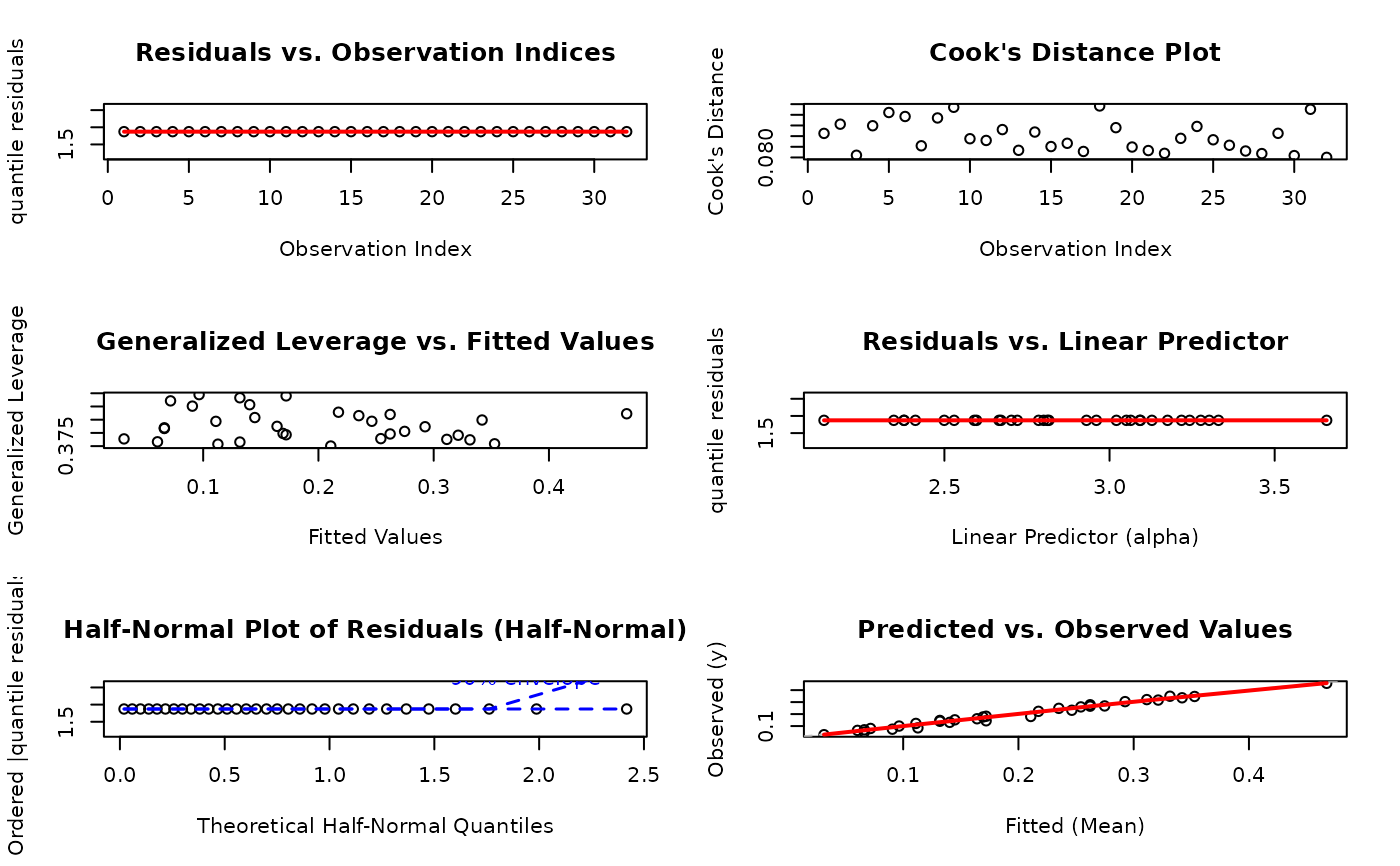 # Example 7.2: Select specific plots
par(mfrow = c(3, 1))
plot(fit, which = c(2, 4, 5)) # Cook's distance, Residuals, Half-normal
#> Simulating envelope ( 100 iterations): .......... Done!
# Example 7.2: Select specific plots
par(mfrow = c(3, 1))
plot(fit, which = c(2, 4, 5)) # Cook's distance, Residuals, Half-normal
#> Simulating envelope ( 100 iterations): .......... Done!
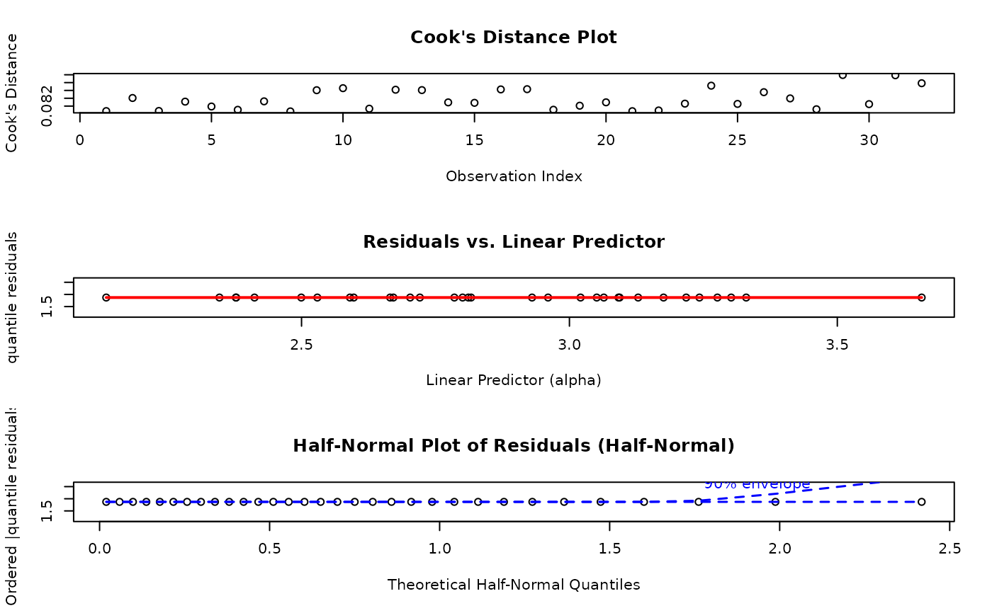 # Example 7.3: Using ggplot2 for modern graphics
plot(fit, use_ggplot = TRUE, arrange_plots = TRUE)
#> Simulating envelope ( 100 iterations): .......... Done!
#> Warning: Removed 1 row containing missing values or values outside the scale range
#> (`geom_segment()`).
# Example 7.3: Using ggplot2 for modern graphics
plot(fit, use_ggplot = TRUE, arrange_plots = TRUE)
#> Simulating envelope ( 100 iterations): .......... Done!
#> Warning: Removed 1 row containing missing values or values outside the scale range
#> (`geom_segment()`).
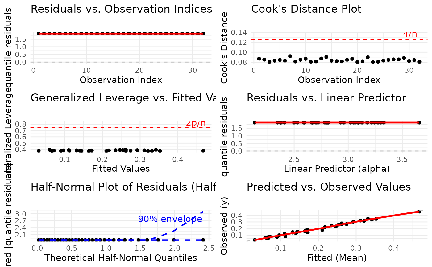 # Example 7.4: Customized half-normal plot
par(mfrow = c(1, 1))
plot(fit,
which = 5,
type = "quantile",
nsim = 200, # More simulations for smoother envelope
level = 0.95
) # 95% confidence envelope
#> Simulating envelope ( 200 iterations): .......... Done!
# Example 7.4: Customized half-normal plot
par(mfrow = c(1, 1))
plot(fit,
which = 5,
type = "quantile",
nsim = 200, # More simulations for smoother envelope
level = 0.95
) # 95% confidence envelope
#> Simulating envelope ( 200 iterations): .......... Done!
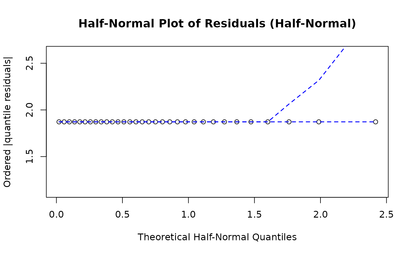 # Example 7.5: Extract diagnostic data programmatically
diagnostics <- plot(fit, save_diagnostics = TRUE)
#> Simulating envelope ( 100 iterations): .......... Done!
head(diagnostics$data) # Residuals, Cook's distance, etc.
#> index y_obs fitted resid abs_resid cook_dist leverage linpred
#> 1 1 0.122 0.10936630 1.873101 1.873101 0.08062570 0.3763283 2.590362
#> 2 2 0.223 0.21750086 1.873101 1.873101 0.08301904 0.3813206 2.960125
#> 3 3 0.347 0.34756539 1.873101 1.873101 0.08443101 0.3842021 3.329888
#> 4 4 0.457 0.46044933 1.873101 1.873101 0.08606928 0.3874881 3.657392
#> 5 5 0.080 0.07061219 1.873101 1.873101 0.08026648 0.3755669 2.412176
#> 6 6 0.131 0.14042911 1.873101 1.873101 0.08500820 0.3853667 2.702704
# SECTION 8: Real Data Example - Food Expenditure
# Load and prepare data
data(FoodExpenditure, package = "betareg")
food_data <- FoodExpenditure
food_data$prop <- food_data$food / food_data$income
# Example 8.1: Basic model
fit_food <- gkwreg(
prop ~ persons | income,
data = food_data,
family = "kw"
)
summary(fit_food)
#>
#> Generalized Kumaraswamy Regression Model Summary
#>
#> Family: kw
#>
#> Call:
#> gkwreg(formula = prop ~ persons | income, data = food_data, family = "kw")
#>
#> Residuals:
#> Min Q1.25% Median Mean Q3.75% Max
#> -0.1668 -0.0417 0.0098 -0.0047 0.0396 0.1527
#>
#> Coefficients:
#> Estimate Std. Error z value Pr(>|z|)
#> alpha:(Intercept) 1.26876 0.14206 8.931 < 2e-16 ***
#> alpha:persons 0.07210 0.01895 3.805 0.000142 ***
#> beta:(Intercept) 3.21312 0.63879 5.030 4.9e-07 ***
#> beta:income 0.03623 0.00922 3.930 8.5e-05 ***
#> ---
#> Signif. codes: 0 ‘***’ 0.001 ‘**’ 0.01 ‘*’ 0.05 ‘.’ 0.1 ‘ ’ 1
#>
#> Confidence intervals (95%):
#> 3% 98%
#> alpha:(Intercept) 0.9903 1.5472
#> alpha:persons 0.0350 0.1092
#> beta:(Intercept) 1.9611 4.4651
#> beta:income 0.0182 0.0543
#>
#> Link functions:
#> alpha: log
#> beta: log
#>
#> Fitted parameter means:
#> alpha: 4.638
#> beta: 244.4
#> gamma: 1
#> delta: 0
#> lambda: 1
#>
#> Model fit statistics:
#> Number of observations: 38
#> Number of parameters: 4
#> Residual degrees of freedom: 34
#> Log-likelihood: 46.34
#> AIC: -84.69
#> BIC: -78.14
#> RMSE: 0.07442
#> Efron's R2: 0.4465
#> Mean Absolute Error: 0.05784
#>
#> Convergence status: Successful
#> Iterations: 18
#>
# Example 8.2: Compare with Beta regression
fit_food_beta <- gkwreg(
prop ~ persons | income,
data = food_data,
family = "beta"
)
# Which fits better?
AIC(fit_food, fit_food_beta)
#> df AIC
#> fit_food 4 -84.68830
#> fit_food_beta 4 -70.28298
# Example 8.3: Model diagnostics
par(mfrow = c(3, 1))
plot(fit_food, which = c(2, 5, 6))
#> Simulating envelope ( 100 iterations): .......... Done!
# Example 7.5: Extract diagnostic data programmatically
diagnostics <- plot(fit, save_diagnostics = TRUE)
#> Simulating envelope ( 100 iterations): .......... Done!
head(diagnostics$data) # Residuals, Cook's distance, etc.
#> index y_obs fitted resid abs_resid cook_dist leverage linpred
#> 1 1 0.122 0.10936630 1.873101 1.873101 0.08062570 0.3763283 2.590362
#> 2 2 0.223 0.21750086 1.873101 1.873101 0.08301904 0.3813206 2.960125
#> 3 3 0.347 0.34756539 1.873101 1.873101 0.08443101 0.3842021 3.329888
#> 4 4 0.457 0.46044933 1.873101 1.873101 0.08606928 0.3874881 3.657392
#> 5 5 0.080 0.07061219 1.873101 1.873101 0.08026648 0.3755669 2.412176
#> 6 6 0.131 0.14042911 1.873101 1.873101 0.08500820 0.3853667 2.702704
# SECTION 8: Real Data Example - Food Expenditure
# Load and prepare data
data(FoodExpenditure, package = "betareg")
food_data <- FoodExpenditure
food_data$prop <- food_data$food / food_data$income
# Example 8.1: Basic model
fit_food <- gkwreg(
prop ~ persons | income,
data = food_data,
family = "kw"
)
summary(fit_food)
#>
#> Generalized Kumaraswamy Regression Model Summary
#>
#> Family: kw
#>
#> Call:
#> gkwreg(formula = prop ~ persons | income, data = food_data, family = "kw")
#>
#> Residuals:
#> Min Q1.25% Median Mean Q3.75% Max
#> -0.1668 -0.0417 0.0098 -0.0047 0.0396 0.1527
#>
#> Coefficients:
#> Estimate Std. Error z value Pr(>|z|)
#> alpha:(Intercept) 1.26876 0.14206 8.931 < 2e-16 ***
#> alpha:persons 0.07210 0.01895 3.805 0.000142 ***
#> beta:(Intercept) 3.21312 0.63879 5.030 4.9e-07 ***
#> beta:income 0.03623 0.00922 3.930 8.5e-05 ***
#> ---
#> Signif. codes: 0 ‘***’ 0.001 ‘**’ 0.01 ‘*’ 0.05 ‘.’ 0.1 ‘ ’ 1
#>
#> Confidence intervals (95%):
#> 3% 98%
#> alpha:(Intercept) 0.9903 1.5472
#> alpha:persons 0.0350 0.1092
#> beta:(Intercept) 1.9611 4.4651
#> beta:income 0.0182 0.0543
#>
#> Link functions:
#> alpha: log
#> beta: log
#>
#> Fitted parameter means:
#> alpha: 4.638
#> beta: 244.4
#> gamma: 1
#> delta: 0
#> lambda: 1
#>
#> Model fit statistics:
#> Number of observations: 38
#> Number of parameters: 4
#> Residual degrees of freedom: 34
#> Log-likelihood: 46.34
#> AIC: -84.69
#> BIC: -78.14
#> RMSE: 0.07442
#> Efron's R2: 0.4465
#> Mean Absolute Error: 0.05784
#>
#> Convergence status: Successful
#> Iterations: 18
#>
# Example 8.2: Compare with Beta regression
fit_food_beta <- gkwreg(
prop ~ persons | income,
data = food_data,
family = "beta"
)
# Which fits better?
AIC(fit_food, fit_food_beta)
#> df AIC
#> fit_food 4 -84.68830
#> fit_food_beta 4 -70.28298
# Example 8.3: Model diagnostics
par(mfrow = c(3, 1))
plot(fit_food, which = c(2, 5, 6))
#> Simulating envelope ( 100 iterations): .......... Done!
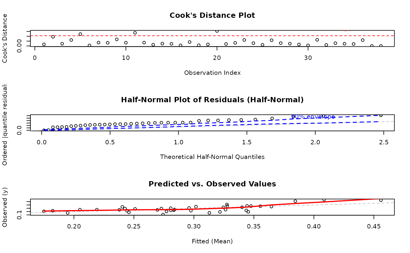 # Example 8.4: Interpretation via effects
# How does proportion spent on food change with income?
income_seq <- seq(min(food_data$income), max(food_data$income), length = 50)
pred_data <- data.frame(
persons = median(food_data$persons),
income = income_seq
)
pred_food <- predict(fit_food, newdata = pred_data, type = "response")
par(mfrow = c(1, 1))
plot(food_data$income, food_data$prop,
xlab = "Income", ylab = "Proportion Spent on Food",
main = "Food Expenditure Pattern"
)
lines(income_seq, pred_food, col = "red", lwd = 2)
# Example 8.4: Interpretation via effects
# How does proportion spent on food change with income?
income_seq <- seq(min(food_data$income), max(food_data$income), length = 50)
pred_data <- data.frame(
persons = median(food_data$persons),
income = income_seq
)
pred_food <- predict(fit_food, newdata = pred_data, type = "response")
par(mfrow = c(1, 1))
plot(food_data$income, food_data$prop,
xlab = "Income", ylab = "Proportion Spent on Food",
main = "Food Expenditure Pattern"
)
lines(income_seq, pred_food, col = "red", lwd = 2)
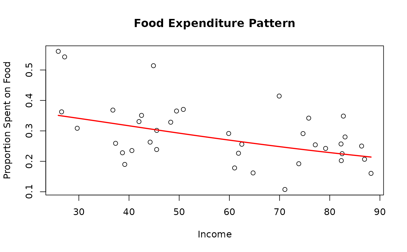 # SECTION 9: Simulation Studies
# Example 9.1: Simple Kumaraswamy simulation
set.seed(123)
n <- 500
x1 <- runif(n, -2, 2)
x2 <- rnorm(n)
# True model: log(alpha) = 0.8 + 0.3*x1, log(beta) = 1.2 - 0.2*x2
eta_alpha <- 0.8 + 0.3 * x1
eta_beta <- 1.2 - 0.2 * x2
alpha_true <- exp(eta_alpha)
beta_true <- exp(eta_beta)
# Generate response
y <- rkw(n, alpha = alpha_true, beta = beta_true)
sim_data <- data.frame(y = y, x1 = x1, x2 = x2)
# Fit and check parameter recovery
fit_sim <- gkwreg(y ~ x1 | x2, data = sim_data, family = "kw")
# Compare estimated vs true coefficients
cbind(
True = c(0.8, 0.3, 1.2, -0.2),
Estimated = coef(fit_sim),
SE = fit_sim$se
)
#> True Estimated SE
#> alpha:(Intercept) 0.8 0.8013394 0.04562729
#> alpha:x1 0.3 0.3011747 0.02418262
#> beta:(Intercept) 1.2 1.1896310 0.07482055
#> beta:x2 -0.2 -0.2419618 0.04607844
# Example 9.2: Complex simulation with all five parameters
set.seed(2203)
n <- 2000
x <- runif(n, -1, 1)
# True parameters
alpha <- exp(0.5 + 0.3 * x)
beta <- exp(1.0 - 0.2 * x)
gamma <- exp(0.7 + 0.4 * x)
delta <- plogis(0.0 + 0.5 * x) # logit scale
lambda <- exp(-0.3 + 0.2 * x)
# Generate from GKw
y <- rgkw(n,
alpha = alpha, beta = beta, gamma = gamma,
delta = delta, lambda = lambda
)
sim_data2 <- data.frame(y = y, x = x)
# Fit GKw model
fit_gkw <- gkwreg(
y ~ x | x | x | x | x,
data = sim_data2,
family = "gkw",
control = gkw_control(method = "L-BFGS-B", maxit = 2000)
)
#> Warning: NaNs produced
summary(fit_gkw)
#>
#> Generalized Kumaraswamy Regression Model Summary
#>
#> Family: gkw
#>
#> Call:
#> gkwreg(formula = y ~ x | x | x | x | x, data = sim_data2, family = "gkw",
#> control = gkw_control(method = "L-BFGS-B", maxit = 2000))
#>
#> Residuals:
#> Min Q1.25% Median Mean Q3.75% Max
#> -0.4583 -0.1645 -0.0606 -0.0450 0.0653 0.6239
#>
#> Coefficients:
#> Estimate Std. Error z value Pr(>|z|)
#> alpha:(Intercept) 0.9380 NaN NaN NaN
#> alpha:x 0.8624 NaN NaN NaN
#> beta:(Intercept) -0.2881 NaN NaN NaN
#> beta:x -0.6939 NaN NaN NaN
#> gamma:(Intercept) 1.5737 NaN NaN NaN
#> gamma:x 1.6823 0.8044 2.091 0.0365 *
#> delta:(Intercept) -0.4862 NaN NaN NaN
#> delta:x 0.9524 0.3335 2.856 0.0043 **
#> lambda:(Intercept) -1.3466 NaN NaN NaN
#> lambda:x -1.3807 0.7270 -1.899 0.0575 .
#> ---
#> Signif. codes: 0 ‘***’ 0.001 ‘**’ 0.01 ‘*’ 0.05 ‘.’ 0.1 ‘ ’ 1
#>
#> Confidence intervals (95%):
#> 3% 98%
#> alpha:(Intercept) NaN NaN
#> alpha:x NaN NaN
#> beta:(Intercept) NaN NaN
#> beta:x NaN NaN
#> gamma:(Intercept) NaN NaN
#> gamma:x 0.1056 3.2590
#> delta:(Intercept) NaN NaN
#> delta:x 0.2987 1.6062
#> lambda:(Intercept) NaN NaN
#> lambda:x -2.8055 0.0441
#>
#> Link functions:
#> alpha: log
#> beta: log
#> gamma: log
#> delta: logit
#> lambda: log
#>
#> Fitted parameter means:
#> alpha: 2.851
#> beta: 0.8156
#> gamma: 7.259
#> delta: 3.863
#> lambda: 0.3538
#>
#> Model fit statistics:
#> Number of observations: 2000
#> Number of parameters: 10
#> Residual degrees of freedom: 1990
#> Log-likelihood: 861.1
#> AIC: -1702
#> BIC: -1646
#> RMSE: 0.1748
#> Efron's R2: 0.301
#> Mean Absolute Error: 0.1428
#>
#> Convergence status: Failed
#> Iterations: 116
#>
# SECTION 10: Handling Convergence Issues
# Example 10.1: Try different optimizers
methods <- c("nlminb", "BFGS", "Nelder-Mead", "CG")
fits_methods <- lapply(methods, function(m) {
tryCatch(
gkwreg(yield ~ batch + temp, GasolineYield,
family = "kw",
control = gkw_control(method = m, silent = TRUE)
),
error = function(e) NULL
)
})
#> Warning: NaNs produced
#> Warning: NaNs produced
names(fits_methods) <- methods
# Check which converged
converged <- sapply(fits_methods, function(f) {
if (is.null(f)) {
return(FALSE)
}
f$convergence
})
print(converged)
#> nlminb BFGS Nelder-Mead CG
#> FALSE TRUE TRUE FALSE
# Example 10.2: Verbose mode for debugging
fit_debug <- gkwreg(
yield ~ batch + temp,
data = GasolineYield,
family = "kw",
control = gkw_control(
method = "BFGS",
silent = TRUE,
trace = 0, # 2, Maximum verbosity
maxit = 1000
)
)
# SECTION 11: Memory and Performance Optimization
# Example 11.1: Minimal object for large datasets
fit_minimal <- gkwreg(
yield ~ batch + temp,
data = GasolineYield,
family = "kw",
model = FALSE, # Don't store model frame
x = FALSE, # Don't store design matrices
y = FALSE, # Don't store response
control = gkw_control(hessian = FALSE) # Skip Hessian
)
# Much smaller object
object.size(fit_minimal)
#> 745256 bytes
# Trade-off: Limited post-fitting capabilities
# Can still use: coef(), logLik(), AIC(), BIC()
# Cannot use: predict(), some diagnostics
# Example 11.2: Fast exploratory analysis
# Fit many models quickly without standard errors
formulas <- list(
yield ~ batch,
yield ~ temp,
yield ~ batch + temp,
yield ~ batch * temp
)
fast_fits <- lapply(formulas, function(f) {
gkwreg(f, GasolineYield,
family = "kw",
control = gkw_control(hessian = FALSE),
model = FALSE, x = FALSE, y = FALSE
)
})
# Compare models via AIC
sapply(fast_fits, AIC)
#> [1] -42.93436 -74.90259 -169.93784 -180.04162
# Refit best model with full inference
best_formula <- formulas[[which.min(sapply(fast_fits, AIC))]]
fit_final <- gkwreg(best_formula, GasolineYield, family = "kw")
#> Warning: NaNs produced
summary(fit_final)
#>
#> Generalized Kumaraswamy Regression Model Summary
#>
#> Family: kw
#>
#> Call:
#> gkwreg(formula = best_formula, data = GasolineYield, family = "kw")
#>
#> Residuals:
#> Min Q1.25% Median Mean Q3.75% Max
#> -33.0040 -32.9155 -32.8540 -32.8354 -32.7615 -32.5750
#>
#> Coefficients:
#> Estimate Std. Error z value Pr(>|z|)
#> alpha:(Intercept) 1.819446 0.007857 231.6 <2e-16 ***
#> alpha:batch1 0.013261 NaN NaN NaN
#> alpha:batch2 -0.263197 NaN NaN NaN
#> alpha:batch3 -0.430252 NaN NaN NaN
#> alpha:batch4 -0.443577 NaN NaN NaN
#> alpha:batch5 -0.991915 NaN NaN NaN
#> alpha:batch6 -0.506689 NaN NaN NaN
#> alpha:batch7 -0.781482 NaN NaN NaN
#> alpha:batch8 -0.986533 NaN NaN NaN
#> alpha:batch9 -0.354264 NaN NaN NaN
#> alpha:temp 0.002835 NaN NaN NaN
#> alpha:batch1:temp 0.002022 NaN NaN NaN
#> alpha:batch2:temp 0.002119 NaN NaN NaN
#> alpha:batch3:temp 0.003146 NaN NaN NaN
#> alpha:batch4:temp 0.002343 NaN NaN NaN
#> alpha:batch5:temp 0.003943 NaN NaN NaN
#> alpha:batch6:temp 0.002479 NaN NaN NaN
#> alpha:batch7:temp 0.002634 NaN NaN NaN
#> alpha:batch8:temp 0.003084 NaN NaN NaN
#> alpha:batch9:temp 0.001238 NaN NaN NaN
#> beta:(Intercept) 35.498475 0.184273 192.6 <2e-16 ***
#> ---
#> Signif. codes: 0 ‘***’ 0.001 ‘**’ 0.01 ‘*’ 0.05 ‘.’ 0.1 ‘ ’ 1
#>
#> Confidence intervals (95%):
#> 3% 98%
#> alpha:(Intercept) 1.8040 1.8348
#> alpha:batch1 NaN NaN
#> alpha:batch2 NaN NaN
#> alpha:batch3 NaN NaN
#> alpha:batch4 NaN NaN
#> alpha:batch5 NaN NaN
#> alpha:batch6 NaN NaN
#> alpha:batch7 NaN NaN
#> alpha:batch8 NaN NaN
#> alpha:batch9 NaN NaN
#> alpha:temp NaN NaN
#> alpha:batch1:temp NaN NaN
#> alpha:batch2:temp NaN NaN
#> alpha:batch3:temp NaN NaN
#> alpha:batch4:temp NaN NaN
#> alpha:batch5:temp NaN NaN
#> alpha:batch6:temp NaN NaN
#> alpha:batch7:temp NaN NaN
#> alpha:batch8:temp NaN NaN
#> alpha:batch9:temp NaN NaN
#> beta:(Intercept) 35.1373 35.8596
#>
#> Link functions:
#> alpha: log
#> beta: log
#>
#> Fitted parameter means:
#> alpha: 22.47
#> beta: 2.608e+15
#> gamma: 1
#> delta: 0
#> lambda: 1
#>
#> Model fit statistics:
#> Number of observations: 32
#> Number of parameters: 21
#> Residual degrees of freedom: 11
#> Log-likelihood: 111
#> AIC: -180
#> BIC: -149.3
#> RMSE: 32.84
#> Efron's R2: -96802
#> Mean Absolute Error: 32.84
#>
#> Convergence status: Failed
#> Iterations: 227
#>
# SECTION 12: Model Selection and Comparison
# Example 12.1: Nested model testing
fit1 <- gkwreg(yield ~ 1, GasolineYield, family = "kw")
fit2 <- gkwreg(yield ~ batch, GasolineYield, family = "kw")
fit3 <- gkwreg(yield ~ batch + temp, GasolineYield, family = "kw")
#> Warning: NaNs produced
# Likelihood ratio tests
anova(fit1, fit2, fit3)
#> Analysis of Deviance Table
#>
#> Model 1: yield ~ 1
#> Model 2: yield ~ batch
#> Model 3: yield ~ batch + temp
#>
#> Resid. Df Resid. Dev Df Deviance Pr(>Chi)
#> fit1 30.00000 -57.02258
#> fit2 21.00000 -64.93436 9 7.91178 0.54306
#> fit3 20.00000 -193.93784 1 129.00348 < 1e-04 ***
#> ---
#> Signif. codes: 0 '***' 0.001 '**' 0.01 '*' 0.05 '.' 0.1 ' ' 1
# Example 12.2: Information criteria table
models <- list(
"Intercept only" = fit1,
"Batch effect" = fit2,
"Batch + Temp" = fit3
)
ic_table <- data.frame(
Model = names(models),
df = sapply(models, function(m) m$npar),
LogLik = sapply(models, logLik),
AIC = sapply(models, AIC),
BIC = sapply(models, BIC),
Delta_AIC = sapply(models, AIC) - min(sapply(models, AIC))
)
print(ic_table)
#> Model df LogLik AIC BIC Delta_AIC
#> Intercept only Intercept only 2 28.51129 -53.02258 -50.09111 116.9153
#> Batch effect Batch effect 11 32.46718 -42.93436 -26.81126 127.0035
#> Batch + Temp Batch + Temp 12 96.96892 -169.93784 -152.34901 0.0000
# Example 12.3: Cross-validation for predictive performance
# 5-fold cross-validation
set.seed(2203)
n <- nrow(GasolineYield)
folds <- sample(rep(1:5, length.out = n))
cv_rmse <- sapply(1:5, function(fold) {
train <- GasolineYield[folds != fold, ]
test <- GasolineYield[folds == fold, ]
fit_train <- gkwreg(yield ~ batch + temp, train,
family = "kw"
)
pred_test <- predict(fit_train, newdata = test, type = "response")
sqrt(mean((test$yield - pred_test)^2))
})
#> Warning: NaNs produced
#> Warning: NaNs produced
#> Warning: NaNs produced
#> Warning: NaNs produced
cat("Cross-validated RMSE:", mean(cv_rmse), "\n")
#> Cross-validated RMSE: 0.09019904
# }
# SECTION 9: Simulation Studies
# Example 9.1: Simple Kumaraswamy simulation
set.seed(123)
n <- 500
x1 <- runif(n, -2, 2)
x2 <- rnorm(n)
# True model: log(alpha) = 0.8 + 0.3*x1, log(beta) = 1.2 - 0.2*x2
eta_alpha <- 0.8 + 0.3 * x1
eta_beta <- 1.2 - 0.2 * x2
alpha_true <- exp(eta_alpha)
beta_true <- exp(eta_beta)
# Generate response
y <- rkw(n, alpha = alpha_true, beta = beta_true)
sim_data <- data.frame(y = y, x1 = x1, x2 = x2)
# Fit and check parameter recovery
fit_sim <- gkwreg(y ~ x1 | x2, data = sim_data, family = "kw")
# Compare estimated vs true coefficients
cbind(
True = c(0.8, 0.3, 1.2, -0.2),
Estimated = coef(fit_sim),
SE = fit_sim$se
)
#> True Estimated SE
#> alpha:(Intercept) 0.8 0.8013394 0.04562729
#> alpha:x1 0.3 0.3011747 0.02418262
#> beta:(Intercept) 1.2 1.1896310 0.07482055
#> beta:x2 -0.2 -0.2419618 0.04607844
# Example 9.2: Complex simulation with all five parameters
set.seed(2203)
n <- 2000
x <- runif(n, -1, 1)
# True parameters
alpha <- exp(0.5 + 0.3 * x)
beta <- exp(1.0 - 0.2 * x)
gamma <- exp(0.7 + 0.4 * x)
delta <- plogis(0.0 + 0.5 * x) # logit scale
lambda <- exp(-0.3 + 0.2 * x)
# Generate from GKw
y <- rgkw(n,
alpha = alpha, beta = beta, gamma = gamma,
delta = delta, lambda = lambda
)
sim_data2 <- data.frame(y = y, x = x)
# Fit GKw model
fit_gkw <- gkwreg(
y ~ x | x | x | x | x,
data = sim_data2,
family = "gkw",
control = gkw_control(method = "L-BFGS-B", maxit = 2000)
)
#> Warning: NaNs produced
summary(fit_gkw)
#>
#> Generalized Kumaraswamy Regression Model Summary
#>
#> Family: gkw
#>
#> Call:
#> gkwreg(formula = y ~ x | x | x | x | x, data = sim_data2, family = "gkw",
#> control = gkw_control(method = "L-BFGS-B", maxit = 2000))
#>
#> Residuals:
#> Min Q1.25% Median Mean Q3.75% Max
#> -0.4583 -0.1645 -0.0606 -0.0450 0.0653 0.6239
#>
#> Coefficients:
#> Estimate Std. Error z value Pr(>|z|)
#> alpha:(Intercept) 0.9380 NaN NaN NaN
#> alpha:x 0.8624 NaN NaN NaN
#> beta:(Intercept) -0.2881 NaN NaN NaN
#> beta:x -0.6939 NaN NaN NaN
#> gamma:(Intercept) 1.5737 NaN NaN NaN
#> gamma:x 1.6823 0.8044 2.091 0.0365 *
#> delta:(Intercept) -0.4862 NaN NaN NaN
#> delta:x 0.9524 0.3335 2.856 0.0043 **
#> lambda:(Intercept) -1.3466 NaN NaN NaN
#> lambda:x -1.3807 0.7270 -1.899 0.0575 .
#> ---
#> Signif. codes: 0 ‘***’ 0.001 ‘**’ 0.01 ‘*’ 0.05 ‘.’ 0.1 ‘ ’ 1
#>
#> Confidence intervals (95%):
#> 3% 98%
#> alpha:(Intercept) NaN NaN
#> alpha:x NaN NaN
#> beta:(Intercept) NaN NaN
#> beta:x NaN NaN
#> gamma:(Intercept) NaN NaN
#> gamma:x 0.1056 3.2590
#> delta:(Intercept) NaN NaN
#> delta:x 0.2987 1.6062
#> lambda:(Intercept) NaN NaN
#> lambda:x -2.8055 0.0441
#>
#> Link functions:
#> alpha: log
#> beta: log
#> gamma: log
#> delta: logit
#> lambda: log
#>
#> Fitted parameter means:
#> alpha: 2.851
#> beta: 0.8156
#> gamma: 7.259
#> delta: 3.863
#> lambda: 0.3538
#>
#> Model fit statistics:
#> Number of observations: 2000
#> Number of parameters: 10
#> Residual degrees of freedom: 1990
#> Log-likelihood: 861.1
#> AIC: -1702
#> BIC: -1646
#> RMSE: 0.1748
#> Efron's R2: 0.301
#> Mean Absolute Error: 0.1428
#>
#> Convergence status: Failed
#> Iterations: 116
#>
# SECTION 10: Handling Convergence Issues
# Example 10.1: Try different optimizers
methods <- c("nlminb", "BFGS", "Nelder-Mead", "CG")
fits_methods <- lapply(methods, function(m) {
tryCatch(
gkwreg(yield ~ batch + temp, GasolineYield,
family = "kw",
control = gkw_control(method = m, silent = TRUE)
),
error = function(e) NULL
)
})
#> Warning: NaNs produced
#> Warning: NaNs produced
names(fits_methods) <- methods
# Check which converged
converged <- sapply(fits_methods, function(f) {
if (is.null(f)) {
return(FALSE)
}
f$convergence
})
print(converged)
#> nlminb BFGS Nelder-Mead CG
#> FALSE TRUE TRUE FALSE
# Example 10.2: Verbose mode for debugging
fit_debug <- gkwreg(
yield ~ batch + temp,
data = GasolineYield,
family = "kw",
control = gkw_control(
method = "BFGS",
silent = TRUE,
trace = 0, # 2, Maximum verbosity
maxit = 1000
)
)
# SECTION 11: Memory and Performance Optimization
# Example 11.1: Minimal object for large datasets
fit_minimal <- gkwreg(
yield ~ batch + temp,
data = GasolineYield,
family = "kw",
model = FALSE, # Don't store model frame
x = FALSE, # Don't store design matrices
y = FALSE, # Don't store response
control = gkw_control(hessian = FALSE) # Skip Hessian
)
# Much smaller object
object.size(fit_minimal)
#> 745256 bytes
# Trade-off: Limited post-fitting capabilities
# Can still use: coef(), logLik(), AIC(), BIC()
# Cannot use: predict(), some diagnostics
# Example 11.2: Fast exploratory analysis
# Fit many models quickly without standard errors
formulas <- list(
yield ~ batch,
yield ~ temp,
yield ~ batch + temp,
yield ~ batch * temp
)
fast_fits <- lapply(formulas, function(f) {
gkwreg(f, GasolineYield,
family = "kw",
control = gkw_control(hessian = FALSE),
model = FALSE, x = FALSE, y = FALSE
)
})
# Compare models via AIC
sapply(fast_fits, AIC)
#> [1] -42.93436 -74.90259 -169.93784 -180.04162
# Refit best model with full inference
best_formula <- formulas[[which.min(sapply(fast_fits, AIC))]]
fit_final <- gkwreg(best_formula, GasolineYield, family = "kw")
#> Warning: NaNs produced
summary(fit_final)
#>
#> Generalized Kumaraswamy Regression Model Summary
#>
#> Family: kw
#>
#> Call:
#> gkwreg(formula = best_formula, data = GasolineYield, family = "kw")
#>
#> Residuals:
#> Min Q1.25% Median Mean Q3.75% Max
#> -33.0040 -32.9155 -32.8540 -32.8354 -32.7615 -32.5750
#>
#> Coefficients:
#> Estimate Std. Error z value Pr(>|z|)
#> alpha:(Intercept) 1.819446 0.007857 231.6 <2e-16 ***
#> alpha:batch1 0.013261 NaN NaN NaN
#> alpha:batch2 -0.263197 NaN NaN NaN
#> alpha:batch3 -0.430252 NaN NaN NaN
#> alpha:batch4 -0.443577 NaN NaN NaN
#> alpha:batch5 -0.991915 NaN NaN NaN
#> alpha:batch6 -0.506689 NaN NaN NaN
#> alpha:batch7 -0.781482 NaN NaN NaN
#> alpha:batch8 -0.986533 NaN NaN NaN
#> alpha:batch9 -0.354264 NaN NaN NaN
#> alpha:temp 0.002835 NaN NaN NaN
#> alpha:batch1:temp 0.002022 NaN NaN NaN
#> alpha:batch2:temp 0.002119 NaN NaN NaN
#> alpha:batch3:temp 0.003146 NaN NaN NaN
#> alpha:batch4:temp 0.002343 NaN NaN NaN
#> alpha:batch5:temp 0.003943 NaN NaN NaN
#> alpha:batch6:temp 0.002479 NaN NaN NaN
#> alpha:batch7:temp 0.002634 NaN NaN NaN
#> alpha:batch8:temp 0.003084 NaN NaN NaN
#> alpha:batch9:temp 0.001238 NaN NaN NaN
#> beta:(Intercept) 35.498475 0.184273 192.6 <2e-16 ***
#> ---
#> Signif. codes: 0 ‘***’ 0.001 ‘**’ 0.01 ‘*’ 0.05 ‘.’ 0.1 ‘ ’ 1
#>
#> Confidence intervals (95%):
#> 3% 98%
#> alpha:(Intercept) 1.8040 1.8348
#> alpha:batch1 NaN NaN
#> alpha:batch2 NaN NaN
#> alpha:batch3 NaN NaN
#> alpha:batch4 NaN NaN
#> alpha:batch5 NaN NaN
#> alpha:batch6 NaN NaN
#> alpha:batch7 NaN NaN
#> alpha:batch8 NaN NaN
#> alpha:batch9 NaN NaN
#> alpha:temp NaN NaN
#> alpha:batch1:temp NaN NaN
#> alpha:batch2:temp NaN NaN
#> alpha:batch3:temp NaN NaN
#> alpha:batch4:temp NaN NaN
#> alpha:batch5:temp NaN NaN
#> alpha:batch6:temp NaN NaN
#> alpha:batch7:temp NaN NaN
#> alpha:batch8:temp NaN NaN
#> alpha:batch9:temp NaN NaN
#> beta:(Intercept) 35.1373 35.8596
#>
#> Link functions:
#> alpha: log
#> beta: log
#>
#> Fitted parameter means:
#> alpha: 22.47
#> beta: 2.608e+15
#> gamma: 1
#> delta: 0
#> lambda: 1
#>
#> Model fit statistics:
#> Number of observations: 32
#> Number of parameters: 21
#> Residual degrees of freedom: 11
#> Log-likelihood: 111
#> AIC: -180
#> BIC: -149.3
#> RMSE: 32.84
#> Efron's R2: -96802
#> Mean Absolute Error: 32.84
#>
#> Convergence status: Failed
#> Iterations: 227
#>
# SECTION 12: Model Selection and Comparison
# Example 12.1: Nested model testing
fit1 <- gkwreg(yield ~ 1, GasolineYield, family = "kw")
fit2 <- gkwreg(yield ~ batch, GasolineYield, family = "kw")
fit3 <- gkwreg(yield ~ batch + temp, GasolineYield, family = "kw")
#> Warning: NaNs produced
# Likelihood ratio tests
anova(fit1, fit2, fit3)
#> Analysis of Deviance Table
#>
#> Model 1: yield ~ 1
#> Model 2: yield ~ batch
#> Model 3: yield ~ batch + temp
#>
#> Resid. Df Resid. Dev Df Deviance Pr(>Chi)
#> fit1 30.00000 -57.02258
#> fit2 21.00000 -64.93436 9 7.91178 0.54306
#> fit3 20.00000 -193.93784 1 129.00348 < 1e-04 ***
#> ---
#> Signif. codes: 0 '***' 0.001 '**' 0.01 '*' 0.05 '.' 0.1 ' ' 1
# Example 12.2: Information criteria table
models <- list(
"Intercept only" = fit1,
"Batch effect" = fit2,
"Batch + Temp" = fit3
)
ic_table <- data.frame(
Model = names(models),
df = sapply(models, function(m) m$npar),
LogLik = sapply(models, logLik),
AIC = sapply(models, AIC),
BIC = sapply(models, BIC),
Delta_AIC = sapply(models, AIC) - min(sapply(models, AIC))
)
print(ic_table)
#> Model df LogLik AIC BIC Delta_AIC
#> Intercept only Intercept only 2 28.51129 -53.02258 -50.09111 116.9153
#> Batch effect Batch effect 11 32.46718 -42.93436 -26.81126 127.0035
#> Batch + Temp Batch + Temp 12 96.96892 -169.93784 -152.34901 0.0000
# Example 12.3: Cross-validation for predictive performance
# 5-fold cross-validation
set.seed(2203)
n <- nrow(GasolineYield)
folds <- sample(rep(1:5, length.out = n))
cv_rmse <- sapply(1:5, function(fold) {
train <- GasolineYield[folds != fold, ]
test <- GasolineYield[folds == fold, ]
fit_train <- gkwreg(yield ~ batch + temp, train,
family = "kw"
)
pred_test <- predict(fit_train, newdata = test, type = "response")
sqrt(mean((test$yield - pred_test)^2))
})
#> Warning: NaNs produced
#> Warning: NaNs produced
#> Warning: NaNs produced
#> Warning: NaNs produced
cat("Cross-validated RMSE:", mean(cv_rmse), "\n")
#> Cross-validated RMSE: 0.09019904
# }