Generalized Kumaraswamy Distribution Random Generation

Generates random deviates from the five-parameter Generalized Kumaraswamy (GKw) distribution defined on the interval (0, 1).

Usage

rgkw(n, alpha, beta, gamma, delta, lambda)

Arguments

n: Number of observations. If length(n) > 1, the length is taken to be the number required. Must be a non-negative integer.
alpha: Shape parameter alpha > 0. Can be a scalar or a vector. Default: 1.0.
beta: Shape parameter beta > 0. Can be a scalar or a vector. Default: 1.0.
gamma: Shape parameter gamma > 0. Can be a scalar or a vector. Default: 1.0.
delta: Shape parameter delta >= 0. Can be a scalar or a vector. Default: 0.0.
lambda: Shape parameter lambda > 0. Can be a scalar or a vector. Default: 1.0.

Value

A vector of length n containing random deviates from the GKw distribution. The length of the result is determined by n and the recycling rule applied to the parameters (alpha, beta, gamma, delta, lambda). Returns NaN if parameters are invalid (e.g., alpha <= 0, beta <= 0, gamma <= 0, delta < 0, lambda <= 0).

Details

The generation method relies on the transformation property: if $V \sim \mathrm{Beta}(\gamma, \delta+1)$, then the random variable X defined as $$ X = \left\{ 1 - \left[ 1 - V^{1/\lambda} \right]^{1/\beta} \right\}^{1/\alpha} $$ follows the GKw($\alpha, \beta, \gamma, \delta, \lambda$) distribution.

The algorithm proceeds as follows:

Generate V from stats::rbeta(n, shape1 = gamma, shape2 = delta + 1).
Calculate $v = V^{1/\lambda}$.
Calculate $w = (1 - v)^{1/\beta}$.
Calculate $x = (1 - w)^{1/\alpha}$.

Parameters (alpha, beta, gamma, delta, lambda) are recycled to match the length required by n. Numerical stability is maintained by handling potential edge cases during the transformations.

References

Cordeiro, G. M., & de Castro, M. (2011). A new family of generalized distributions. Journal of Statistical Computation and Simulation

Kumaraswamy, P. (1980). A generalized probability density function for double-bounded random processes. Journal of Hydrology, 46(1-2), 79-88.

Author

Lopes, J. E.

Examples

# \donttest{
set.seed(1234) # for reproducibility

# Generate 1000 random values from a specific GKw distribution (Kw case)
x_sample <- rgkw(1000, alpha = 2, beta = 3, gamma = 1, delta = 0, lambda = 1)
summary(x_sample)
#>    Min. 1st Qu.  Median    Mean 3rd Qu.    Max. 
#> 0.01524 0.31493 0.46345 0.46265 0.60804 0.96441 

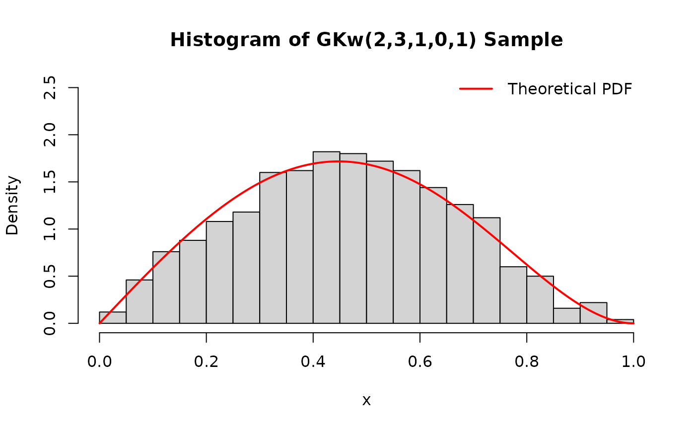
# Histogram of generated values compared to theoretical density
hist(x_sample, breaks = 30, freq = FALSE, # freq=FALSE for density scale
     main = "Histogram of GKw(2,3,1,0,1) Sample", xlab = "x", ylim = c(0, 2.5))
curve(dgkw(x, alpha = 2, beta = 3, gamma = 1, delta = 0, lambda = 1),
      add = TRUE, col = "red", lwd = 2, n = 201)
legend("topright", legend = "Theoretical PDF", col = "red", lwd = 2, bty = "n")


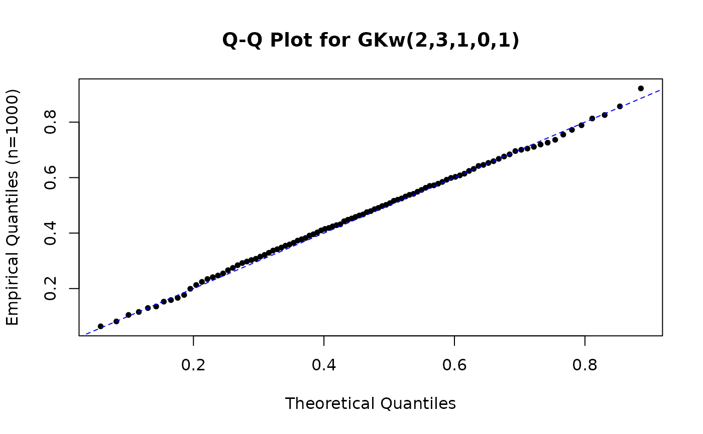
# Comparing empirical and theoretical quantiles (Q-Q plot)
prob_points <- seq(0.01, 0.99, by = 0.01)
theo_quantiles <- qgkw(prob_points, alpha = 2, beta = 3, gamma = 1, delta = 0, lambda = 1)
emp_quantiles <- quantile(x_sample, prob_points)

plot(theo_quantiles, emp_quantiles, pch = 16, cex = 0.8,
     main = "Q-Q Plot for GKw(2,3,1,0,1)",
     xlab = "Theoretical Quantiles", ylab = "Empirical Quantiles (n=1000)")
abline(a = 0, b = 1, col = "blue", lty = 2)


# Using vectorized parameters: generate 1 value for each alpha
alphas_vec <- c(0.5, 1.0, 2.0)
n_param <- length(alphas_vec)
samples_vec <- rgkw(n_param, alpha = alphas_vec, beta = 2, gamma = 1, delta = 0, lambda = 1)
print(samples_vec) # One sample for each alpha value
#> [1] 0.4386491 0.2135709 0.8667377
# Result length matches n=3, parameters alpha recycled accordingly

# Example with invalid parameters (should produce NaN)
invalid_sample <- rgkw(1, alpha = -1, beta = 2, gamma = 1, delta = 0, lambda = 1)
#> Warning: rgkw: invalid parameters at index 1 (alpha,beta,gamma>0, delta>=0, lambda>0)
print(invalid_sample)
#> [1] NA
# }