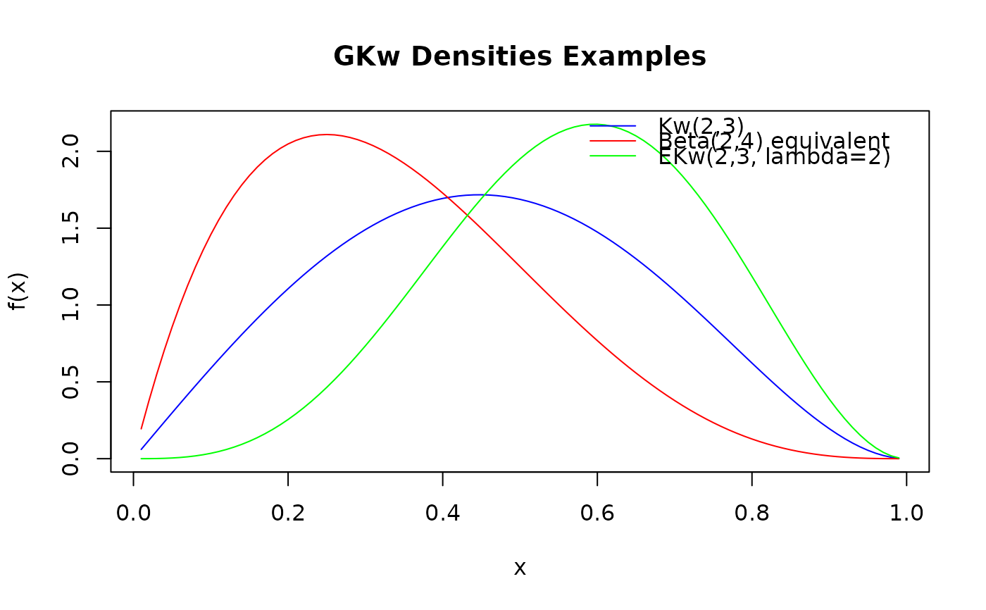
Density of the Generalized Kumaraswamy Distribution

Computes the probability density function (PDF) for the five-parameter Generalized Kumaraswamy (GKw) distribution, defined on the interval (0, 1).

Usage

dgkw(x, alpha = 1, beta = 1, gamma = 1, delta = 0, lambda = 1, log = FALSE)

Arguments

x: Vector of quantiles (values between 0 and 1).
alpha: Shape parameter alpha > 0. Can be a scalar or a vector. Default: 1.0.
beta: Shape parameter beta > 0. Can be a scalar or a vector. Default: 1.0.
gamma: Shape parameter gamma > 0. Can be a scalar or a vector. Default: 1.0.
delta: Shape parameter delta >= 0. Can be a scalar or a vector. Default: 0.0.
lambda: Shape parameter lambda > 0. Can be a scalar or a vector. Default: 1.0.
log: Logical; if TRUE, the logarithm of the density is returned. Default: FALSE.

Value

A vector of density values ($f(x)$) or log-density values ($\log(f(x))$). The length of the result is determined by the recycling rule applied to the arguments (x, alpha, beta, gamma, delta, lambda). Returns 0 (or -Inf if log = TRUE) for x strictly outside the interval [0, 1]. At the closed boundaries x = 0 and x = 1 the limiting density is returned rather than 0, following the convention of base R's density functions (compare dbeta); depending on the parameters that limit is 0, a finite positive value, or Inf. An out-of-bound or missing parameter is an error, not a return value: the wrapper stops with a message naming the parameter. An infinite parameter is not currently intercepted there and reaches the C++ layer, which treats it as invalid.

Details

The probability density function of the Generalized Kumaraswamy (GKw) distribution with parameters alpha ($\alpha$), beta ($\beta$), gamma ($\gamma$), delta ($\delta$), and lambda ($\lambda$) is given by: $$ f(x; \alpha, \beta, \gamma, \delta, \lambda) = \frac{\lambda \alpha \beta x^{\alpha-1}(1-x^{\alpha})^{\beta-1}} {B(\gamma, \delta+1)} [1-(1-x^{\alpha})^{\beta}]^{\gamma\lambda-1} [1-[1-(1-x^{\alpha})^{\beta}]^{\lambda}]^{\delta} $$ for $x \in (0,1)$, where $B(a, b)$ is the Beta function beta.

This distribution was proposed by Carrasco, Ferrari & Cordeiro (2010) and includes several other distributions as special cases:

Kumaraswamy (Kw): gamma = 1, delta = 0, lambda = 1
Exponentiated Kumaraswamy (EKw): gamma = 1, delta = 0
Beta-Kumaraswamy (BKw): lambda = 1
Generalized Beta type 1 (GB1 - implies McDonald): alpha = 1, beta = 1
Beta distribution: alpha = 1, beta = 1, lambda = 1

The function includes checks for valid parameters and input values x. It uses numerical stabilization for x close to 0 or 1.

References

Carrasco, J. M. F., Ferrari, S. L. P., & Cordeiro, G. M. (2010). A new generalized Kumaraswamy distribution. arXiv preprint arXiv:1004.0911. doi:10.48550/arXiv.1004.0911

Cordeiro, G. M., & de Castro, M. (2011). A new family of generalized distributions. Journal of Statistical Computation and Simulation, 81(7), 883-898. doi:10.1080/00949650903530745

Kumaraswamy, P. (1980). A generalized probability density function for double-bounded random processes. Journal of Hydrology, 46(1-2), 79-88. doi:10.1016/0022-1694(80)90036-0

Author

Lopes, J. E.

Examples

x <- c(0.1, 0.3, 0.5, 0.7, 0.9)
dgkw(x, alpha = 2, beta = 3, gamma = 1.5, delta = 0.5, lambda = 1.2)
#> [1] 0.10703949 1.33993326 2.30916136 1.18032685 0.05372826
dgkw(x, alpha = 2, beta = 3, gamma = 1.5, delta = 0.5, lambda = 1.2, log = TRUE)
#> [1] -2.2345574  0.2926198  0.8368844  0.1657914 -2.9238161

## Kumaraswamy is GKw with gamma = 1, delta = 0, lambda = 1 (the defaults)
all.equal(dgkw(x, alpha = 2, beta = 3), dkw(x, alpha = 2, beta = 3))
#> [1] TRUE

## Beta(gamma, delta + 1) is GKw with alpha = beta = lambda = 1
all.equal(dgkw(x, gamma = 2, delta = 3), stats::dbeta(x, 2, 4))
#> [1] TRUE

## The density integrates to one
integrate(dgkw, 0, 1, alpha = 2, beta = 3, gamma = 1.5, delta = 0.5,
    lambda = 1.2, rel.tol = 1e-10)
#> 1 with absolute error < 4.1e-11

curve(dgkw(x, alpha = 2, beta = 3, gamma = 1.5, delta = 0.5, lambda = 1.2),
    from = 0, to = 1, ylab = "density")