Random Number Generation for the Kumaraswamy (Kw) Distribution

Generates random deviates from the two-parameter Kumaraswamy (Kw) distribution with shape parameters alpha ($\alpha$) and beta ($\beta$).

Usage

rkw(n, alpha, beta)

Arguments

n: Number of observations. If length(n) > 1, the length is taken to be the number required. Must be a non-negative integer.
alpha: Shape parameter alpha > 0. Can be a scalar or a vector. Default: 1.0.
beta: Shape parameter beta > 0. Can be a scalar or a vector. Default: 1.0.

Value

A vector of length n containing random deviates from the Kw distribution, with values in (0, 1). The length of the result is determined by n and the recycling rule applied to the parameters (alpha, beta). Returns NaN if parameters are invalid (e.g., alpha <= 0, beta <= 0).

Details

The generation method uses the inverse transform (quantile) method. That is, if $U$ is a random variable following a standard Uniform distribution on (0, 1), then $X = Q(U)$ follows the Kw distribution, where $Q(p)$ is the Kw quantile function (qkw): $$ Q(p) = \left\{ 1 - (1 - p)^{1/\beta} \right\}^{1/\alpha} $$ The implementation generates $U$ using runif and applies this transformation. This is equivalent to the general GKw generation method (rgkw) evaluated at $\gamma=1, \delta=0, \lambda=1$.

References

Kumaraswamy, P. (1980). A generalized probability density function for double-bounded random processes. Journal of Hydrology, 46(1-2), 79-88.

Jones, M. C. (2009). Kumaraswamy's distribution: A beta-type distribution with some tractability advantages. Statistical Methodology, 6(1), 70-81.

Devroye, L. (1986). Non-Uniform Random Variate Generation. Springer-Verlag. (General methods for random variate generation).

Author

Lopes, J. E.

Examples

# \donttest{
set.seed(2029) # for reproducibility

# Generate 1000 random values from a specific Kw distribution
alpha_par <- 2.0
beta_par <- 3.0

x_sample_kw <- rkw(1000, alpha = alpha_par, beta = beta_par)
summary(x_sample_kw)
#>    Min. 1st Qu.  Median    Mean 3rd Qu.    Max. 
#> 0.01825 0.29985 0.45247 0.45264 0.58978 0.93608 

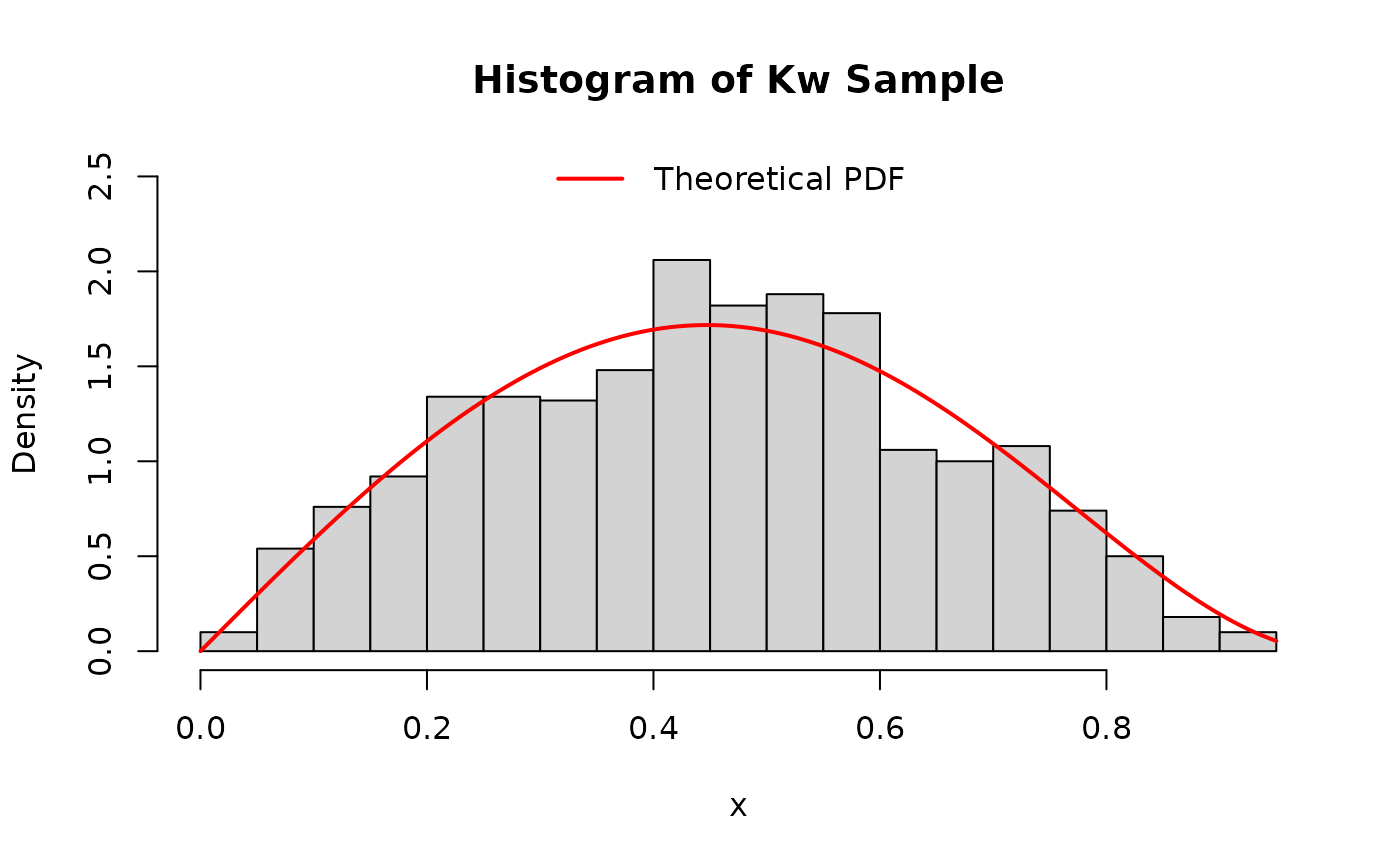
# Histogram of generated values compared to theoretical density
hist(x_sample_kw, breaks = 30, freq = FALSE, # freq=FALSE for density
     main = "Histogram of Kw Sample", xlab = "x", ylim = c(0, 2.5))
curve(dkw(x, alpha = alpha_par, beta = beta_par),
      add = TRUE, col = "red", lwd = 2, n = 201)
legend("top", legend = "Theoretical PDF", col = "red", lwd = 2, bty = "n")


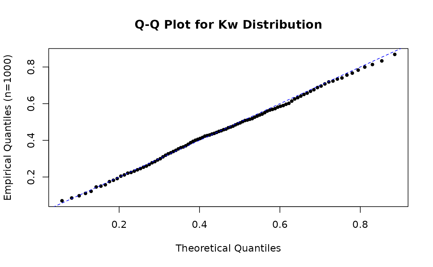
# Comparing empirical and theoretical quantiles (Q-Q plot)
prob_points <- seq(0.01, 0.99, by = 0.01)
theo_quantiles <- qkw(prob_points, alpha = alpha_par, beta = beta_par)
emp_quantiles <- quantile(x_sample_kw, prob_points, type = 7)

plot(theo_quantiles, emp_quantiles, pch = 16, cex = 0.8,
     main = "Q-Q Plot for Kw Distribution",
     xlab = "Theoretical Quantiles", ylab = "Empirical Quantiles (n=1000)")
abline(a = 0, b = 1, col = "blue", lty = 2)


# Compare summary stats with rgkw(..., gamma=1, delta=0, lambda=1)
# Note: individual values will differ due to randomness
x_sample_gkw <- rgkw(1000, alpha = alpha_par, beta = beta_par, gamma = 1.0,
                     delta = 0.0, lambda = 1.0)
print("Summary stats for rkw sample:")
#> [1] "Summary stats for rkw sample:"
print(summary(x_sample_kw))
#>    Min. 1st Qu.  Median    Mean 3rd Qu.    Max. 
#> 0.01825 0.29985 0.45247 0.45264 0.58978 0.93608 
print("Summary stats for rgkw(gamma=1, delta=0, lambda=1) sample:")
#> [1] "Summary stats for rgkw(gamma=1, delta=0, lambda=1) sample:"
print(summary(x_sample_gkw)) # Should be similar
#>    Min. 1st Qu.  Median    Mean 3rd Qu.    Max. 
#> 0.00568 0.30017 0.45069 0.45469 0.59646 0.95381 

# }