Cumulative Distribution Function (CDF) of the Kumaraswamy (Kw) Distribution

Computes the cumulative distribution function (CDF), $P(X \le q)$, for the two-parameter Kumaraswamy (Kw) distribution with shape parameters alpha ($\alpha$) and beta ($\beta$). This distribution is defined on the interval (0, 1).

Usage

pkw(q, alpha, beta, lower_tail = TRUE, log_p = FALSE)

Arguments

q: Vector of quantiles (values generally between 0 and 1).
alpha: Shape parameter alpha > 0. Can be a scalar or a vector. Default: 1.0.
beta: Shape parameter beta > 0. Can be a scalar or a vector. Default: 1.0.
lower_tail: Logical; if TRUE (default), probabilities are $P(X \le q)$, otherwise, $P(X > q)$.
log_p: Logical; if TRUE, probabilities $p$ are given as $\log(p)$. Default: FALSE.

Value

A vector of probabilities, $F(q)$, or their logarithms/complements depending on lower_tail and log_p. The length of the result is determined by the recycling rule applied to the arguments (q, alpha, beta). Returns 0 (or -Inf if log_p = TRUE) for q <= 0 and 1 (or 0 if log_p = TRUE) for q >= 1. Returns NaN for invalid parameters.

Details

The cumulative distribution function (CDF) of the Kumaraswamy (Kw) distribution is given by: $$ F(x; \alpha, \beta) = 1 - (1 - x^\alpha)^\beta $$ for $0 < x < 1$, $\alpha > 0$, and $\beta > 0$.

The Kw distribution is a special case of several generalized distributions:

Generalized Kumaraswamy (pgkw) with $\gamma=1, \delta=0, \lambda=1$.
Exponentiated Kumaraswamy (pekw) with $\lambda=1$.
Kumaraswamy-Kumaraswamy (pkkw) with $\delta=0, \lambda=1$.

The implementation uses the closed-form expression for efficiency.

References

Kumaraswamy, P. (1980). A generalized probability density function for double-bounded random processes. Journal of Hydrology, 46(1-2), 79-88.

Jones, M. C. (2009). Kumaraswamy's distribution: A beta-type distribution with some tractability advantages. Statistical Methodology, 6(1), 70-81.

Author

Lopes, J. E.

Examples

# \donttest{
# Example values
q_vals <- c(0.2, 0.5, 0.8)
alpha_par <- 2.0
beta_par <- 3.0

# Calculate CDF P(X <= q) using pkw
probs <- pkw(q_vals, alpha_par, beta_par)
print(probs)
#> [1] 0.115264 0.578125 0.953344

# Calculate upper tail P(X > q)
probs_upper <- pkw(q_vals, alpha_par, beta_par, lower_tail = FALSE)
print(probs_upper)
#> [1] 0.884736 0.421875 0.046656
# Check: probs + probs_upper should be 1
print(probs + probs_upper)
#> [1] 1 1 1

# Calculate log CDF
log_probs <- pkw(q_vals, alpha_par, beta_par, log_p = TRUE)
print(log_probs)
#> [1] -2.16053013 -0.54796517 -0.04777948
# Check: should match log(probs)
print(log(probs))
#> [1] -2.16053013 -0.54796517 -0.04777948

# Compare with pgkw setting gamma = 1, delta = 0, lambda = 1
probs_gkw <- pgkw(q_vals, alpha_par, beta_par, gamma = 1.0, delta = 0.0,
                  lambda = 1.0)
print(paste("Max difference:", max(abs(probs - probs_gkw)))) # Should be near zero
#> [1] "Max difference: 1.11022302462516e-16"

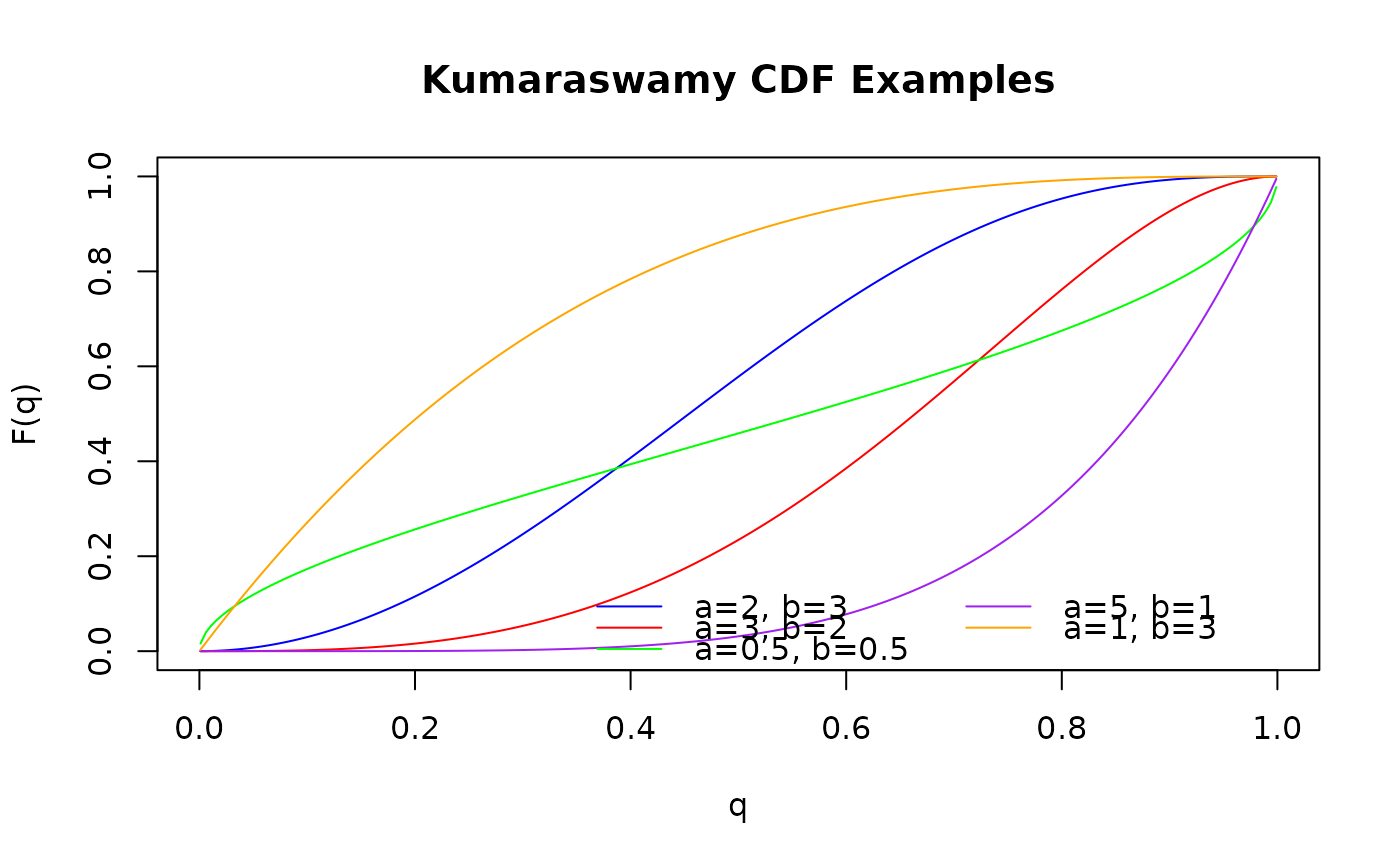
# Plot the CDF for different shape parameter combinations
curve_q <- seq(0.001, 0.999, length.out = 200)
plot(curve_q, pkw(curve_q, alpha = 2, beta = 3), type = "l",
     main = "Kumaraswamy CDF Examples", xlab = "q", ylab = "F(q)",
     col = "blue", ylim = c(0, 1))
lines(curve_q, pkw(curve_q, alpha = 3, beta = 2), col = "red")
lines(curve_q, pkw(curve_q, alpha = 0.5, beta = 0.5), col = "green")
lines(curve_q, pkw(curve_q, alpha = 5, beta = 1), col = "purple")
lines(curve_q, pkw(curve_q, alpha = 1, beta = 3), col = "orange")
legend("bottomright", legend = c("a=2, b=3", "a=3, b=2", "a=0.5, b=0.5", "a=5, b=1", "a=1, b=3"),
       col = c("blue", "red", "green", "purple", "orange"), lty = 1, bty = "n", ncol = 2)


# }