Cumulative Distribution Function (CDF) of the EKw Distribution

Computes the cumulative distribution function (CDF), $P(X \le q)$, for the Exponentiated Kumaraswamy (EKw) distribution with parameters alpha ($\alpha$), beta ($\beta$), and lambda ($\lambda$). This distribution is defined on the interval (0, 1) and is a special case of the Generalized Kumaraswamy (GKw) distribution where $\gamma = 1$ and $\delta = 0$.

Usage

pekw(q, alpha, beta, lambda, lower_tail = TRUE, log_p = FALSE)

Arguments

q: Vector of quantiles (values generally between 0 and 1).
alpha: Shape parameter alpha > 0. Can be a scalar or a vector. Default: 1.0.
beta: Shape parameter beta > 0. Can be a scalar or a vector. Default: 1.0.
lambda: Shape parameter lambda > 0 (exponent parameter). Can be a scalar or a vector. Default: 1.0.
lower_tail: Logical; if TRUE (default), probabilities are $P(X \le q)$, otherwise, $P(X > q)$.
log_p: Logical; if TRUE, probabilities $p$ are given as $\log(p)$. Default: FALSE.

Value

A vector of probabilities, $F(q)$, or their logarithms/complements depending on lower_tail and log_p. The length of the result is determined by the recycling rule applied to the arguments (q, alpha, beta, lambda). Returns 0 (or -Inf if log_p = TRUE) for q <= 0 and 1 (or 0 if log_p = TRUE) for q >= 1. Returns NaN for invalid parameters.

Details

The Exponentiated Kumaraswamy (EKw) distribution is a special case of the five-parameter Generalized Kumaraswamy distribution (pgkw) obtained by setting parameters $\gamma = 1$ and $\delta = 0$.

The CDF of the GKw distribution is $F_{GKw}(q) = I_{y(q)}(\gamma, \delta+1)$, where $y(q) = [1-(1-q^{\alpha})^{\beta}]^{\lambda}$ and $I_x(a,b)$ is the regularized incomplete beta function (pbeta). Setting $\gamma=1$ and $\delta=0$ gives $I_{y(q)}(1, 1)$. Since $I_x(1, 1) = x$, the CDF simplifies to $y(q)$: $$ F(q; \alpha, \beta, \lambda) = \bigl[1 - (1 - q^\alpha)^\beta \bigr]^\lambda $$ for $0 < q < 1$. The implementation uses this closed-form expression for efficiency and handles lower_tail and log_p arguments appropriately.

References

Nadarajah, S., Cordeiro, G. M., & Ortega, E. M. (2012). The exponentiated Kumaraswamy distribution. Journal of the Franklin Institute, 349(3),

Cordeiro, G. M., & de Castro, M. (2011). A new family of generalized distributions. Journal of Statistical Computation and Simulation,

Kumaraswamy, P. (1980). A generalized probability density function for double-bounded random processes. Journal of Hydrology, 46(1-2), 79-88.

Author

Lopes, J. E.

Examples

# \donttest{
# Example values
q_vals <- c(0.2, 0.5, 0.8)
alpha_par <- 2.0
beta_par <- 3.0
lambda_par <- 1.5

# Calculate CDF P(X <= q)
probs <- pekw(q_vals, alpha_par, beta_par, lambda_par)
print(probs)
#> [1] 0.03913276 0.43957464 0.93083875

# Calculate upper tail P(X > q)
probs_upper <- pekw(q_vals, alpha_par, beta_par, lambda_par,
                    lower_tail = FALSE)
print(probs_upper)
#> [1] 0.96086724 0.56042536 0.06916125
# Check: probs + probs_upper should be 1
print(probs + probs_upper)
#> [1] 1 1 1

# Calculate log CDF
log_probs <- pekw(q_vals, alpha_par, beta_par, lambda_par, log_p = TRUE)
print(log_probs)
#> [1] -3.24079519 -0.82194776 -0.07166921
# Check: should match log(probs)
print(log(probs))
#> [1] -3.24079519 -0.82194776 -0.07166921

# Compare with pgkw setting gamma = 1, delta = 0
probs_gkw <- pgkw(q_vals, alpha_par, beta_par, gamma = 1.0, delta = 0.0,
                 lambda = lambda_par)
print(paste("Max difference:", max(abs(probs - probs_gkw)))) # Should be near zero
#> [1] "Max difference: 5.55111512312578e-17"

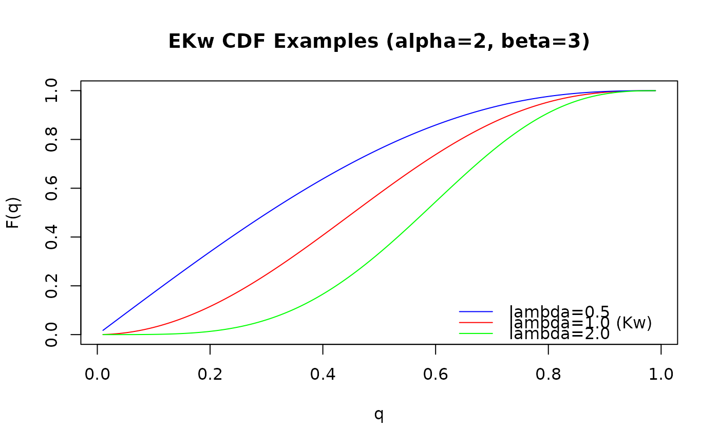
# Plot the CDF for different lambda values
curve_q <- seq(0.01, 0.99, length.out = 200)
curve_p1 <- pekw(curve_q, alpha = 2, beta = 3, lambda = 0.5)
curve_p2 <- pekw(curve_q, alpha = 2, beta = 3, lambda = 1.0) # standard Kw
curve_p3 <- pekw(curve_q, alpha = 2, beta = 3, lambda = 2.0)

plot(curve_q, curve_p2, type = "l", main = "EKw CDF Examples (alpha=2, beta=3)",
     xlab = "q", ylab = "F(q)", col = "red", ylim = c(0, 1))
lines(curve_q, curve_p1, col = "blue")
lines(curve_q, curve_p3, col = "green")
legend("bottomright", legend = c("lambda=0.5", "lambda=1.0 (Kw)", "lambda=2.0"),
       col = c("blue", "red", "green"), lty = 1, bty = "n")

# }