Random Number Generation for the Exponentiated Kumaraswamy (EKw) Distribution

Generates random deviates from the Exponentiated Kumaraswamy (EKw) distribution with parameters alpha ($\alpha$), beta ($\beta$), and lambda ($\lambda$). This distribution is a special case of the Generalized Kumaraswamy (GKw) distribution where $\gamma = 1$ and $\delta = 0$.

Usage

rekw(n, alpha, beta, lambda)

Arguments

n: Number of observations. If length(n) > 1, the length is taken to be the number required. Must be a non-negative integer.
alpha: Shape parameter alpha > 0. Can be a scalar or a vector. Default: 1.0.
beta: Shape parameter beta > 0. Can be a scalar or a vector. Default: 1.0.
lambda: Shape parameter lambda > 0 (exponent parameter). Can be a scalar or a vector. Default: 1.0.

Value

A vector of length n containing random deviates from the EKw distribution. The length of the result is determined by n and the recycling rule applied to the parameters (alpha, beta, lambda). Returns NaN if parameters are invalid (e.g., alpha <= 0, beta <= 0, lambda <= 0).

Details

The generation method uses the inverse transform (quantile) method. That is, if $U$ is a random variable following a standard Uniform distribution on (0, 1), then $X = Q(U)$ follows the EKw distribution, where $Q(u)$ is the EKw quantile function (qekw): $$ Q(u) = \left\{ 1 - \left[ 1 - u^{1/\lambda} \right]^{1/\beta} \right\}^{1/\alpha} $$ This is computationally equivalent to the general GKw generation method (rgkw) when specialized for $\gamma=1, \delta=0$, as the required Beta(1, 1) random variate is equivalent to a standard Uniform(0, 1) variate. The implementation generates $U$ using runif and applies the transformation above.

References

Nadarajah, S., Cordeiro, G. M., & Ortega, E. M. (2012). The exponentiated Kumaraswamy distribution. Journal of the Franklin Institute, 349(3),

Cordeiro, G. M., & de Castro, M. (2011). A new family of generalized distributions. Journal of Statistical Computation and Simulation,

Kumaraswamy, P. (1980). A generalized probability density function for double-bounded random processes. Journal of Hydrology, 46(1-2), 79-88.

Devroye, L. (1986). Non-Uniform Random Variate Generation. Springer-Verlag. (General methods for random variate generation).

Author

Lopes, J. E.

Examples

# \donttest{
set.seed(2027) # for reproducibility

# Generate 1000 random values from a specific EKw distribution
alpha_par <- 2.0
beta_par <- 3.0
lambda_par <- 1.5

x_sample_ekw <- rekw(1000, alpha = alpha_par, beta = beta_par, lambda = lambda_par)
summary(x_sample_ekw)
#>    Min. 1st Qu.  Median    Mean 3rd Qu.    Max. 
#> 0.01796 0.40449 0.53117 0.52906 0.65941 0.95165 

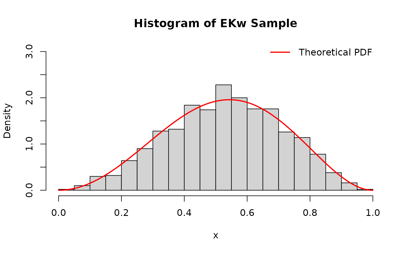
# Histogram of generated values compared to theoretical density
hist(x_sample_ekw, breaks = 30, freq = FALSE, # freq=FALSE for density
     main = "Histogram of EKw Sample", xlab = "x", ylim = c(0, 3.0))
curve(dekw(x, alpha = alpha_par, beta = beta_par, lambda = lambda_par),
      add = TRUE, col = "red", lwd = 2, n = 201)
legend("topright", legend = "Theoretical PDF", col = "red", lwd = 2, bty = "n")


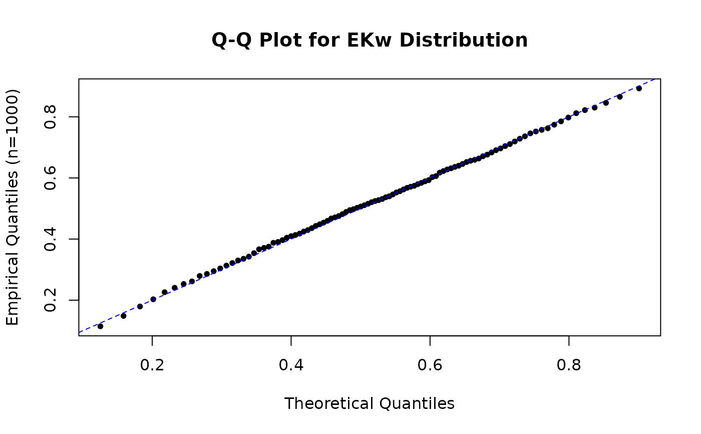
# Comparing empirical and theoretical quantiles (Q-Q plot)
prob_points <- seq(0.01, 0.99, by = 0.01)
theo_quantiles <- qekw(prob_points, alpha = alpha_par, beta = beta_par,
                       lambda = lambda_par)
emp_quantiles <- quantile(x_sample_ekw, prob_points, type = 7)

plot(theo_quantiles, emp_quantiles, pch = 16, cex = 0.8,
     main = "Q-Q Plot for EKw Distribution",
     xlab = "Theoretical Quantiles", ylab = "Empirical Quantiles (n=1000)")
abline(a = 0, b = 1, col = "blue", lty = 2)


# Compare summary stats with rgkw(..., gamma=1, delta=0, ...)
# Note: individual values will differ due to randomness
x_sample_gkw <- rgkw(1000, alpha = alpha_par, beta = beta_par, gamma = 1.0,
                     delta = 0.0, lambda = lambda_par)
print("Summary stats for rekw sample:")
#> [1] "Summary stats for rekw sample:"
print(summary(x_sample_ekw))
#>    Min. 1st Qu.  Median    Mean 3rd Qu.    Max. 
#> 0.01796 0.40449 0.53117 0.52906 0.65941 0.95165 
print("Summary stats for rgkw(gamma=1, delta=0) sample:")
#> [1] "Summary stats for rgkw(gamma=1, delta=0) sample:"
print(summary(x_sample_gkw)) # Should be similar
#>    Min. 1st Qu.  Median    Mean 3rd Qu.    Max. 
#> 0.02851 0.39394 0.53074 0.52923 0.66914 0.98175 

# }