Density of the Exponentiated Kumaraswamy (EKw) Distribution

Computes the probability density function (PDF) for the Exponentiated Kumaraswamy (EKw) distribution with parameters alpha ($\alpha$), beta ($\beta$), and lambda ($\lambda$). This distribution is defined on the interval (0, 1).

Usage

dekw(x, alpha, beta, lambda, log_prob = FALSE)

Arguments

x: Vector of quantiles (values between 0 and 1).
alpha: Shape parameter alpha > 0. Can be a scalar or a vector. Default: 1.0.
beta: Shape parameter beta > 0. Can be a scalar or a vector. Default: 1.0.
lambda: Shape parameter lambda > 0 (exponent parameter). Can be a scalar or a vector. Default: 1.0.
log_prob: Logical; if TRUE, the logarithm of the density is returned ($\log(f(x))$). Default: FALSE.

Value

A vector of density values ($f(x)$) or log-density values ($\log(f(x))$). The length of the result is determined by the recycling rule applied to the arguments (x, alpha, beta, lambda). Returns 0 (or -Inf if log_prob = TRUE) for x outside the interval (0, 1), or NaN if parameters are invalid (e.g., alpha <= 0, beta <= 0, lambda <= 0).

Details

The probability density function (PDF) of the Exponentiated Kumaraswamy (EKw) distribution is given by: $$ f(x; \alpha, \beta, \lambda) = \lambda \alpha \beta x^{\alpha-1} (1 - x^\alpha)^{\beta-1} \bigl[1 - (1 - x^\alpha)^\beta \bigr]^{\lambda - 1} $$ for $0 < x < 1$.

The EKw distribution is a special case of the five-parameter Generalized Kumaraswamy (GKw) distribution (dgkw) obtained by setting the parameters $\gamma = 1$ and $\delta = 0$. When $\lambda = 1$, the EKw distribution reduces to the standard Kumaraswamy distribution.

References

Nadarajah, S., Cordeiro, G. M., & Ortega, E. M. (2012). The exponentiated Kumaraswamy distribution. Journal of the Franklin Institute, 349(3),

Cordeiro, G. M., & de Castro, M. (2011). A new family of generalized distributions. Journal of Statistical Computation and Simulation,

Kumaraswamy, P. (1980). A generalized probability density function for double-bounded random processes. Journal of Hydrology, 46(1-2), 79-88.

Author

Lopes, J. E.

Examples

# \donttest{
# Example values
x_vals <- c(0.2, 0.5, 0.8)
alpha_par <- 2.0
beta_par <- 3.0
lambda_par <- 1.5 # Exponent parameter

# Calculate density
densities <- dekw(x_vals, alpha_par, beta_par, lambda_par)
print(densities)
#> [1] 0.5631989 1.9246241 0.9110922

# Calculate log-density
log_densities <- dekw(x_vals, alpha_par, beta_par, lambda_par, log_prob = TRUE)
print(log_densities)
#> [1] -0.57412239  0.65473067 -0.09311121
# Check: should match log(densities)
print(log(densities))
#> [1] -0.57412239  0.65473067 -0.09311121

# Compare with dgkw setting gamma = 1, delta = 0
densities_gkw <- dgkw(x_vals, alpha_par, beta_par, gamma = 1.0, delta = 0.0,
                      lambda = lambda_par)
print(paste("Max difference:", max(abs(densities - densities_gkw)))) # Should be near zero
#> [1] "Max difference: 3.33066907387547e-16"

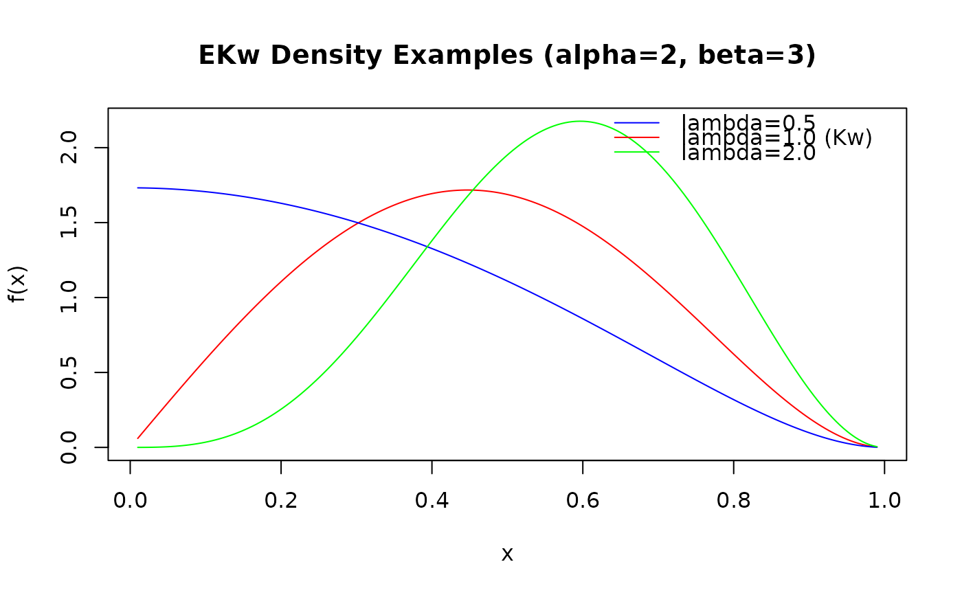
# Plot the density for different lambda values
curve_x <- seq(0.01, 0.99, length.out = 200)
curve_y1 <- dekw(curve_x, alpha = 2, beta = 3, lambda = 0.5) # less peaked
curve_y2 <- dekw(curve_x, alpha = 2, beta = 3, lambda = 1.0) # standard Kw
curve_y3 <- dekw(curve_x, alpha = 2, beta = 3, lambda = 2.0) # more peaked

plot(curve_x, curve_y2, type = "l", main = "EKw Density Examples (alpha=2, beta=3)",
     xlab = "x", ylab = "f(x)", col = "red", ylim = range(0, curve_y1, curve_y2, curve_y3))
lines(curve_x, curve_y1, col = "blue")
lines(curve_x, curve_y3, col = "green")
legend("topright", legend = c("lambda=0.5", "lambda=1.0 (Kw)", "lambda=2.0"),
       col = c("blue", "red", "green"), lty = 1, bty = "n")

# }