Density of the Kumaraswamy (Kw) Distribution

Computes the probability density function (PDF) for the two-parameter Kumaraswamy (Kw) distribution with shape parameters alpha ($\alpha$) and beta ($\beta$). This distribution is defined on the interval (0, 1).

Usage

dkw(x, alpha, beta, log_prob = FALSE)

Arguments

x: Vector of quantiles (values between 0 and 1).
alpha: Shape parameter alpha > 0. Can be a scalar or a vector. Default: 1.0.
beta: Shape parameter beta > 0. Can be a scalar or a vector. Default: 1.0.
log_prob: Logical; if TRUE, the logarithm of the density is returned ($\log(f(x))$). Default: FALSE.

Value

A vector of density values ($f(x)$) or log-density values ($\log(f(x))$). The length of the result is determined by the recycling rule applied to the arguments (x, alpha, beta). Returns 0 (or -Inf if log_prob = TRUE) for x outside the interval (0, 1), or NaN if parameters are invalid (e.g., alpha <= 0, beta <= 0).

Details

The probability density function (PDF) of the Kumaraswamy (Kw) distribution is given by: $$ f(x; \alpha, \beta) = \alpha \beta x^{\alpha-1} (1 - x^\alpha)^{\beta-1} $$ for $0 < x < 1$, $\alpha > 0$, and $\beta > 0$.

The Kumaraswamy distribution is identical to the Generalized Kumaraswamy (GKw) distribution (dgkw) with parameters $\gamma = 1$, $\delta = 0$, and $\lambda = 1$. It is also a special case of the Exponentiated Kumaraswamy (dekw) with $\lambda = 1$, and the Kumaraswamy-Kumaraswamy (dkkw) with $\delta = 0$ and $\lambda = 1$.

References

Kumaraswamy, P. (1980). A generalized probability density function for double-bounded random processes. Journal of Hydrology, 46(1-2), 79-88.

Jones, M. C. (2009). Kumaraswamy's distribution: A beta-type distribution with some tractability advantages. Statistical Methodology, 6(1), 70-81.

Author

Lopes, J. E.

Examples

# \donttest{
# Example values
x_vals <- c(0.2, 0.5, 0.8)
alpha_par <- 2.0
beta_par <- 3.0

# Calculate density using dkw
densities <- dkw(x_vals, alpha_par, beta_par)
print(densities)
#> [1] 1.10592 1.68750 0.62208

# Calculate log-density
log_densities <- dkw(x_vals, alpha_par, beta_par, log_prob = TRUE)
print(log_densities)
#> [1]  0.1006776  0.5232481 -0.4746866
# Check: should match log(densities)
print(log(densities))
#> [1]  0.1006776  0.5232481 -0.4746866

# Compare with dgkw setting gamma = 1, delta = 0, lambda = 1
densities_gkw <- dgkw(x_vals, alpha_par, beta_par, gamma = 1.0, delta = 0.0,
                      lambda = 1.0)
print(paste("Max difference:", max(abs(densities - densities_gkw)))) # Should be near zero
#> [1] "Max difference: 2.22044604925031e-16"

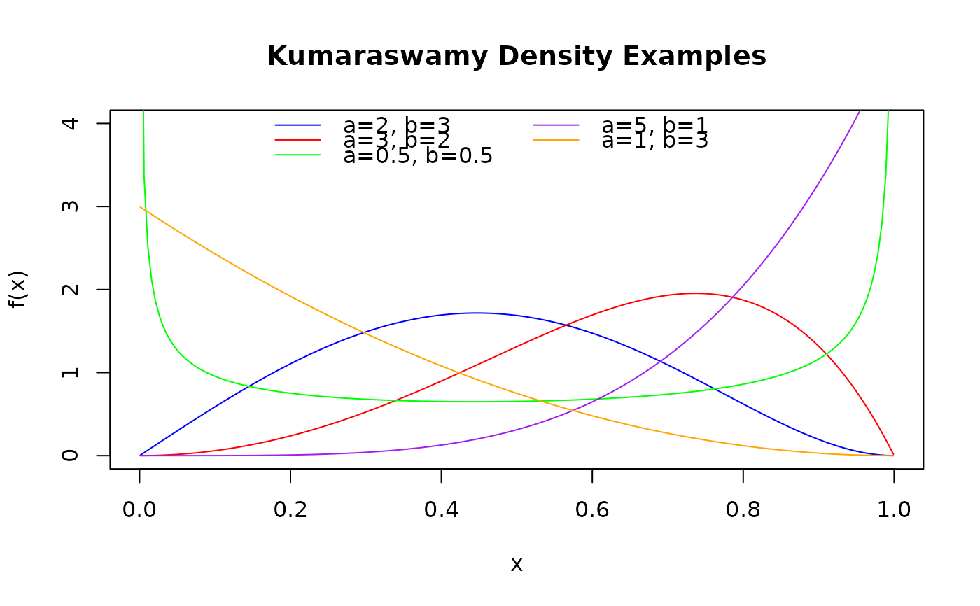
# Plot the density for different shape parameter combinations
curve_x <- seq(0.001, 0.999, length.out = 200)
plot(curve_x, dkw(curve_x, alpha = 2, beta = 3), type = "l",
     main = "Kumaraswamy Density Examples", xlab = "x", ylab = "f(x)",
     col = "blue", ylim = c(0, 4))
lines(curve_x, dkw(curve_x, alpha = 3, beta = 2), col = "red")
lines(curve_x, dkw(curve_x, alpha = 0.5, beta = 0.5), col = "green") # U-shaped
lines(curve_x, dkw(curve_x, alpha = 5, beta = 1), col = "purple") # J-shaped
lines(curve_x, dkw(curve_x, alpha = 1, beta = 3), col = "orange") # J-shaped (reversed)
legend("top", legend = c("a=2, b=3", "a=3, b=2", "a=0.5, b=0.5", "a=5, b=1", "a=1, b=3"),
       col = c("blue", "red", "green", "purple", "orange"), lty = 1, bty = "n", ncol = 2)

# }