Density of the Kumaraswamy-Kumaraswamy (KKw) Distribution

Computes the probability density function (PDF) for the Kumaraswamy-Kumaraswamy (KKw) distribution with parameters alpha ($\alpha$), beta ($\beta$), delta ($\delta$), and lambda ($\lambda$). This distribution is defined on the interval (0, 1).

Usage

dkkw(x, alpha = 1, beta = 1, delta = 0, lambda = 1, log = FALSE)

Arguments

x: Vector of quantiles (values between 0 and 1).
alpha: Shape parameter alpha > 0. Can be a scalar or a vector. Default: 1.0.
beta: Shape parameter beta > 0. Can be a scalar or a vector. Default: 1.0.
delta: Shape parameter delta >= 0. Can be a scalar or a vector. Default: 0.0.
lambda: Shape parameter lambda > 0. Can be a scalar or a vector. Default: 1.0.
log: Logical; if TRUE, the logarithm of the density is returned ($\log(f(x))$). Default: FALSE.

Value

A vector of density values ($f(x)$) or log-density values ($\log(f(x))$). The length of the result is determined by the recycling rule applied to the arguments (x, alpha, beta, delta, lambda). Returns 0 (or -Inf if log = TRUE) for x strictly outside the interval [0, 1]. At the closed boundaries x = 0 and x = 1 the limiting density is returned rather than 0, following the convention of base R's density functions (compare dbeta); depending on the parameters that limit is 0, a finite positive value, or Inf. An out-of-bound or missing parameter is an error, not a return value: the wrapper stops with a message naming the parameter. An infinite parameter is not currently intercepted there and reaches the C++ layer, which treats it as invalid.

Details

The Kumaraswamy-Kumaraswamy (KKw) distribution is a special case of the five-parameter Generalized Kumaraswamy distribution (dgkw) obtained by setting the parameter $\gamma = 1$.

The probability density function is given by: $$ f(x; \alpha, \beta, \delta, \lambda) = (\delta + 1) \lambda \alpha \beta x^{\alpha - 1} (1 - x^\alpha)^{\beta - 1} \bigl[1 - (1 - x^\alpha)^\beta\bigr]^{\lambda - 1} \bigl\{1 - \bigl[1 - (1 - x^\alpha)^\beta\bigr]^\lambda\bigr\}^{\delta} $$ for $0 < x < 1$. Note that $1/(\delta+1)$ corresponds to the Beta function term $B(1, \delta+1)$ when $\gamma=1$.

Numerical evaluation follows similar stability considerations as dgkw.

References

Cordeiro, G. M., & de Castro, M. (2011). A new family of generalized distributions. Journal of Statistical Computation and Simulation, 81(7), 883-898. doi:10.1080/00949650903530745

Kumaraswamy, P. (1980). A generalized probability density function for double-bounded random processes. Journal of Hydrology, 46(1-2), 79-88. doi:10.1016/0022-1694(80)90036-0

Author

Lopes, J. E.

Examples

x <- c(0.1, 0.3, 0.5, 0.7, 0.9)
dkkw(x, alpha = 2, beta = 3, delta = 0.5, lambda = 1.2)
#> [1] 0.52003496 1.82902324 1.88969788 0.75724620 0.03177953
dkkw(x, alpha = 2, beta = 3, delta = 0.5, lambda = 1.2, log = TRUE)
#> [1] -0.6538592  0.6037821  0.6364170 -0.2780669 -3.4489331

## KKw is GKw with gamma = 1
all.equal(dkkw(x, 2, 3, 0.5, 1.2), dgkw(x, 2, 3, gamma = 1, delta = 0.5,
    lambda = 1.2))
#> [1] TRUE

## The density integrates to one
integrate(dkkw, 0, 1, alpha = 2, beta = 3, delta = 0.5, lambda = 1.2,
    rel.tol = 1e-10)
#> 1 with absolute error < 9.6e-13

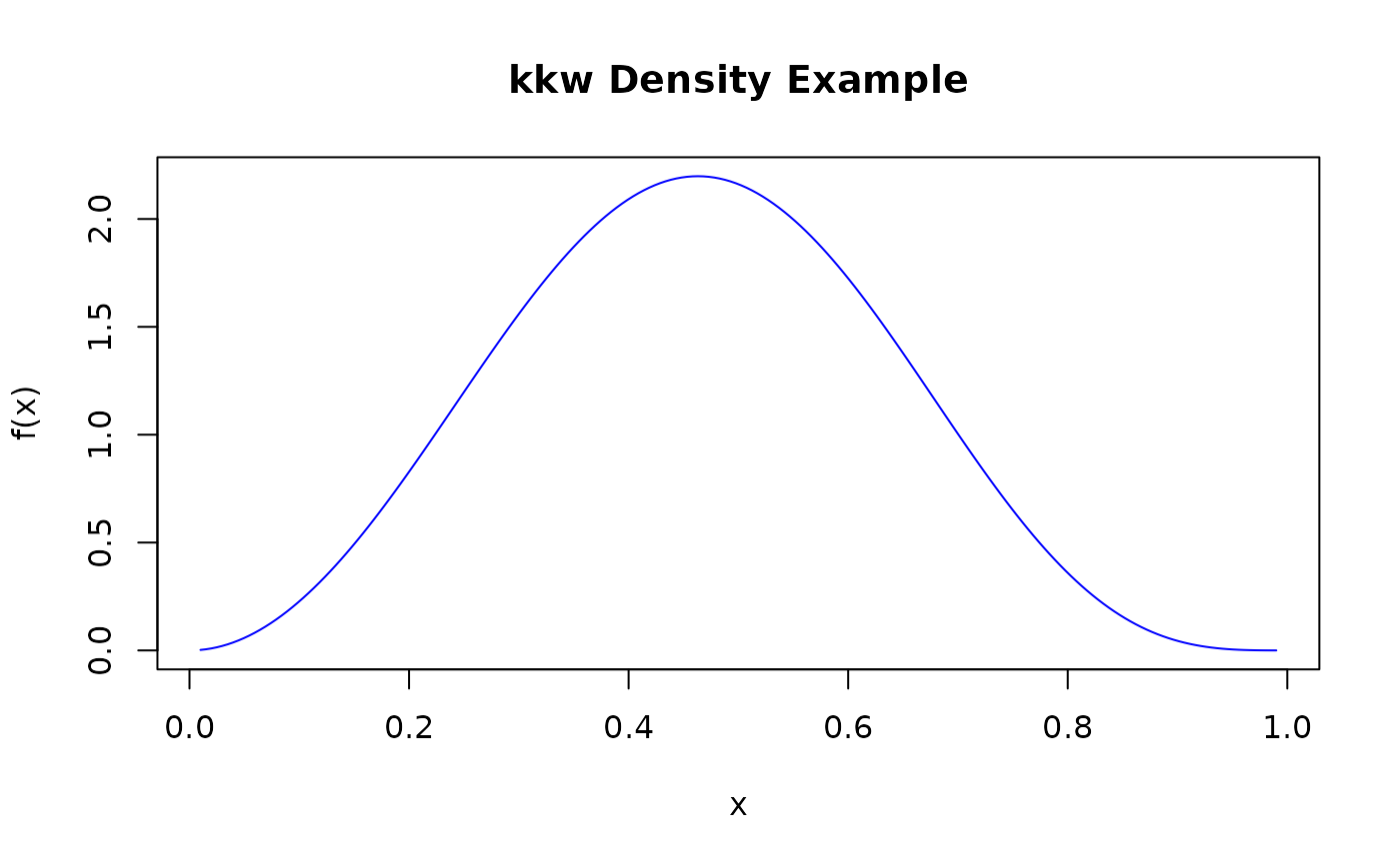
curve(dkkw(x, alpha = 2, beta = 3, delta = 0.5, lambda = 1.2), from = 0,
    to = 1, ylab = "density")