Computes the negative log-likelihood function for the Beta-Kumaraswamy (BKw)
distribution with parameters alpha (\(\alpha\)), beta
(\(\beta\)), gamma (\(\gamma\)), and delta (\(\delta\)),
given a vector of observations. This distribution is the special case of the
Generalized Kumaraswamy (GKw) distribution where \(\lambda = 1\). This function
is typically used for maximum likelihood estimation via numerical optimization.
Value
Returns a single double value representing the negative
log-likelihood (\(-\ell(\theta|\mathbf{x})\)). Returns Inf
if any parameter values in par are invalid according to their
constraints, or if any value in data is not in the interval (0, 1).
Details
The Beta-Kumaraswamy (BKw) distribution is the GKw distribution (dgkw)
with \(\lambda=1\). Its probability density function (PDF) is:
$$
f(x | \theta) = \frac{\alpha \beta}{B(\gamma, \delta+1)} x^{\alpha - 1} \bigl(1 - x^\alpha\bigr)^{\beta(\delta+1) - 1} \bigl[1 - \bigl(1 - x^\alpha\bigr)^\beta\bigr]^{\gamma - 1}
$$
for \(0 < x < 1\), \(\theta = (\alpha, \beta, \gamma, \delta)\), and \(B(a,b)\)
is the Beta function (beta).
The log-likelihood function \(\ell(\theta | \mathbf{x})\) for a sample
\(\mathbf{x} = (x_1, \dots, x_n)\) is \(\sum_{i=1}^n \ln f(x_i | \theta)\):
$$
\ell(\theta | \mathbf{x}) = n[\ln(\alpha) + \ln(\beta) - \ln B(\gamma, \delta+1)]
+ \sum_{i=1}^{n} [(\alpha-1)\ln(x_i) + (\beta(\delta+1)-1)\ln(v_i) + (\gamma-1)\ln(w_i)]
$$
where:
\(v_i = 1 - x_i^{\alpha}\)
\(w_i = 1 - v_i^{\beta} = 1 - (1-x_i^{\alpha})^{\beta}\)
This function computes and returns the negative log-likelihood, \(-\ell(\theta|\mathbf{x})\),
suitable for minimization using optimization routines like optim.
Numerical stability is maintained similarly to llgkw.
References
Cordeiro, G. M., & de Castro, M. (2011). A new family of generalized distributions. Journal of Statistical Computation and Simulation
Kumaraswamy, P. (1980). A generalized probability density function for double-bounded random processes. Journal of Hydrology, 46(1-2), 79-88.
Examples
# \donttest{
## Example 1: Basic Log-Likelihood Evaluation
# Generate sample data
set.seed(2203)
n <- 1000
true_params <- c(alpha = 2.0, beta = 1.5, gamma = 1.5, delta = 0.5)
data <- rbkw(n,
alpha = true_params[1], beta = true_params[2],
gamma = true_params[3], delta = true_params[4]
)
# Evaluate negative log-likelihood at true parameters
nll_true <- llbkw(par = true_params, data = data)
cat("Negative log-likelihood at true parameters:", nll_true, "\n")
#> Negative log-likelihood at true parameters: -268.3902
# Evaluate at different parameter values
test_params <- rbind(
c(1.5, 1.0, 1.0, 0.3),
c(2.0, 1.5, 1.5, 0.5),
c(2.5, 2.0, 2.0, 0.7)
)
nll_values <- apply(test_params, 1, function(p) llbkw(p, data))
results <- data.frame(
Alpha = test_params[, 1],
Beta = test_params[, 2],
Gamma = test_params[, 3],
Delta = test_params[, 4],
NegLogLik = nll_values
)
print(results, digits = 4)
#> Alpha Beta Gamma Delta NegLogLik
#> 1 1.5 1.0 1.0 0.3 -145.5
#> 2 2.0 1.5 1.5 0.5 -268.4
#> 3 2.5 2.0 2.0 0.7 -162.6
## Example 2: Maximum Likelihood Estimation
# Optimization using BFGS with no analytical gradient
fit <- optim(
par = c(0.5, 1, 1.1, 0.3),
fn = llbkw,
# gr = grbkw,
data = data,
method = "BFGS",
control = list(maxit = 2000),
hessian = TRUE
)
mle <- fit$par
names(mle) <- c("alpha", "beta", "gamma", "delta")
se <- sqrt(diag(solve(fit$hessian)))
results <- data.frame(
Parameter = c("alpha", "beta", "gamma", "delta"),
True = true_params,
MLE = mle,
SE = se,
CI_Lower = mle - 1.96 * se,
CI_Upper = mle + 1.96 * se
)
print(results, digits = 4)
#> Parameter True MLE SE CI_Lower CI_Upper
#> alpha alpha 2.0 2.51814 0.7598 1.0289 4.007
#> beta beta 1.5 2.36884 4.5438 -6.5369 11.275
#> gamma gamma 1.5 1.15021 0.4206 0.3259 1.975
#> delta delta 0.5 0.04261 2.0140 -3.9048 3.990
cat("\nNegative log-likelihood at MLE:", fit$value, "\n")
#>
#> Negative log-likelihood at MLE: -270.2379
cat("AIC:", 2 * fit$value + 2 * length(mle), "\n")
#> AIC: -532.4758
cat("BIC:", 2 * fit$value + length(mle) * log(n), "\n")
#> BIC: -512.8448
## Example 3: Comparing Optimization Methods
methods <- c("BFGS", "L-BFGS-B", "Nelder-Mead", "CG")
start_params <- c(1.8, 1.2, 1.1, 0.3)
comparison <- data.frame(
Method = character(),
Alpha = numeric(),
Beta = numeric(),
Gamma = numeric(),
Delta = numeric(),
NegLogLik = numeric(),
Convergence = integer(),
stringsAsFactors = FALSE
)
for (method in methods) {
if (method %in% c("BFGS", "CG")) {
fit_temp <- optim(
par = start_params,
fn = llbkw,
gr = grbkw,
data = data,
method = method
)
} else if (method == "L-BFGS-B") {
fit_temp <- optim(
par = start_params,
fn = llbkw,
gr = grbkw,
data = data,
method = method,
lower = c(0.01, 0.01, 0.01, 0.01),
upper = c(100, 100, 100, 100)
)
} else {
fit_temp <- optim(
par = start_params,
fn = llbkw,
data = data,
method = method
)
}
comparison <- rbind(comparison, data.frame(
Method = method,
Alpha = fit_temp$par[1],
Beta = fit_temp$par[2],
Gamma = fit_temp$par[3],
Delta = fit_temp$par[4],
NegLogLik = fit_temp$value,
Convergence = fit_temp$convergence,
stringsAsFactors = FALSE
))
}
print(comparison, digits = 4, row.names = FALSE)
#> Method Alpha Beta Gamma Delta NegLogLik Convergence
#> BFGS 2.528 2.470 1.145 0.0001526 -270.2 0
#> L-BFGS-B 2.526 2.446 1.146 0.0100000 -270.2 0
#> Nelder-Mead 2.570 2.332 1.122 0.0670160 -270.2 1
#> CG 2.516 1.618 1.147 0.5412596 -270.2 1
## Example 4: Likelihood Ratio Test
# Test H0: delta = 0.5 vs H1: delta free
loglik_full <- -fit$value
restricted_ll <- function(params_restricted, data, delta_fixed) {
llbkw(par = c(
params_restricted[1], params_restricted[2],
params_restricted[3], delta_fixed
), data = data)
}
fit_restricted <- optim(
par = mle[1:3],
fn = restricted_ll,
data = data,
delta_fixed = 0.5,
method = "Nelder-Mead"
)
loglik_restricted <- -fit_restricted$value
lr_stat <- 2 * (loglik_full - loglik_restricted)
p_value <- pchisq(lr_stat, df = 1, lower.tail = FALSE)
cat("LR Statistic:", round(lr_stat, 4), "\n")
#> LR Statistic: 0.0492
cat("P-value:", format.pval(p_value, digits = 4), "\n")
#> P-value: 0.8244
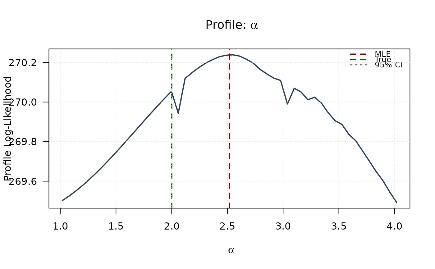
## Example 5: Univariate Profile Likelihoods
# Profile for alpha
alpha_grid <- seq(mle[1] - 1.5, mle[1] + 1.5, length.out = 50)
alpha_grid <- alpha_grid[alpha_grid > 0]
profile_ll_alpha <- numeric(length(alpha_grid))
for (i in seq_along(alpha_grid)) {
profile_fit <- optim(
par = mle[-1],
fn = function(p) llbkw(c(alpha_grid[i], p), data),
method = "Nelder-Mead"
)
profile_ll_alpha[i] <- -profile_fit$value
}
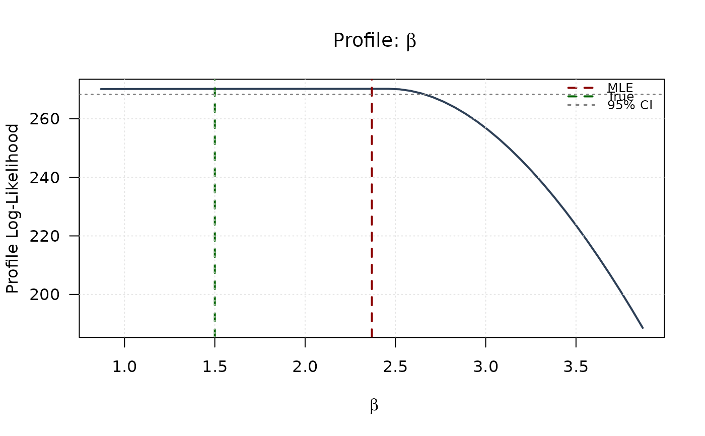
# Profile for beta
beta_grid <- seq(mle[2] - 1.5, mle[2] + 1.5, length.out = 50)
beta_grid <- beta_grid[beta_grid > 0]
profile_ll_beta <- numeric(length(beta_grid))
for (i in seq_along(beta_grid)) {
profile_fit <- optim(
par = c(mle[1], mle[3], mle[4]),
fn = function(p) llbkw(c(mle[1], beta_grid[i], p[1], p[2]), data),
method = "Nelder-Mead"
)
profile_ll_beta[i] <- -profile_fit$value
}
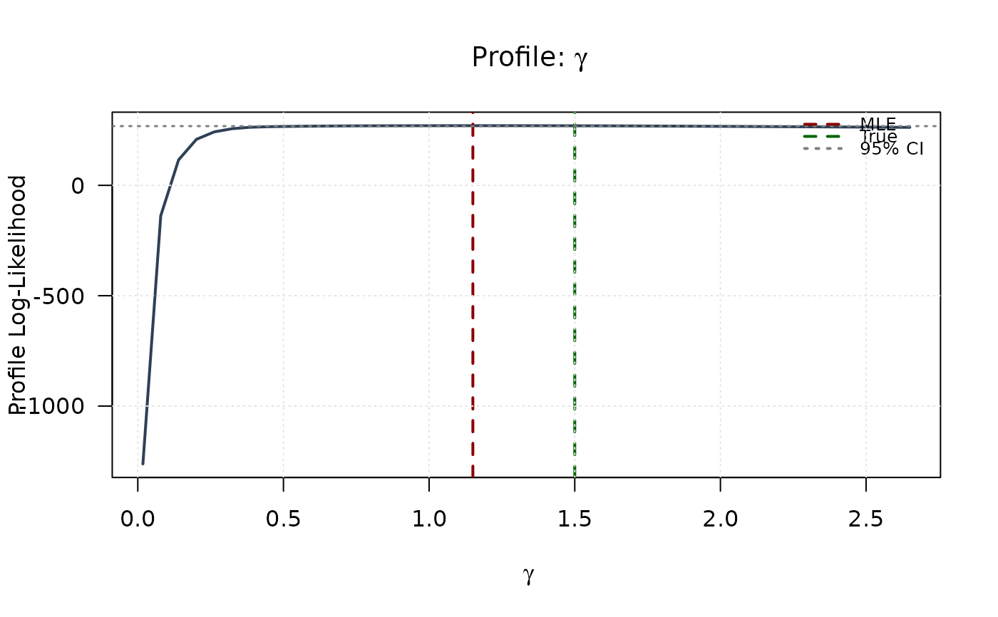
# Profile for gamma
gamma_grid <- seq(mle[3] - 1.5, mle[3] + 1.5, length.out = 50)
gamma_grid <- gamma_grid[gamma_grid > 0]
profile_ll_gamma <- numeric(length(gamma_grid))
for (i in seq_along(gamma_grid)) {
profile_fit <- optim(
par = c(mle[1], mle[2], mle[4]),
fn = function(p) llbkw(c(p[1], mle[2], gamma_grid[i], p[2]), data),
method = "Nelder-Mead"
)
profile_ll_gamma[i] <- -profile_fit$value
}
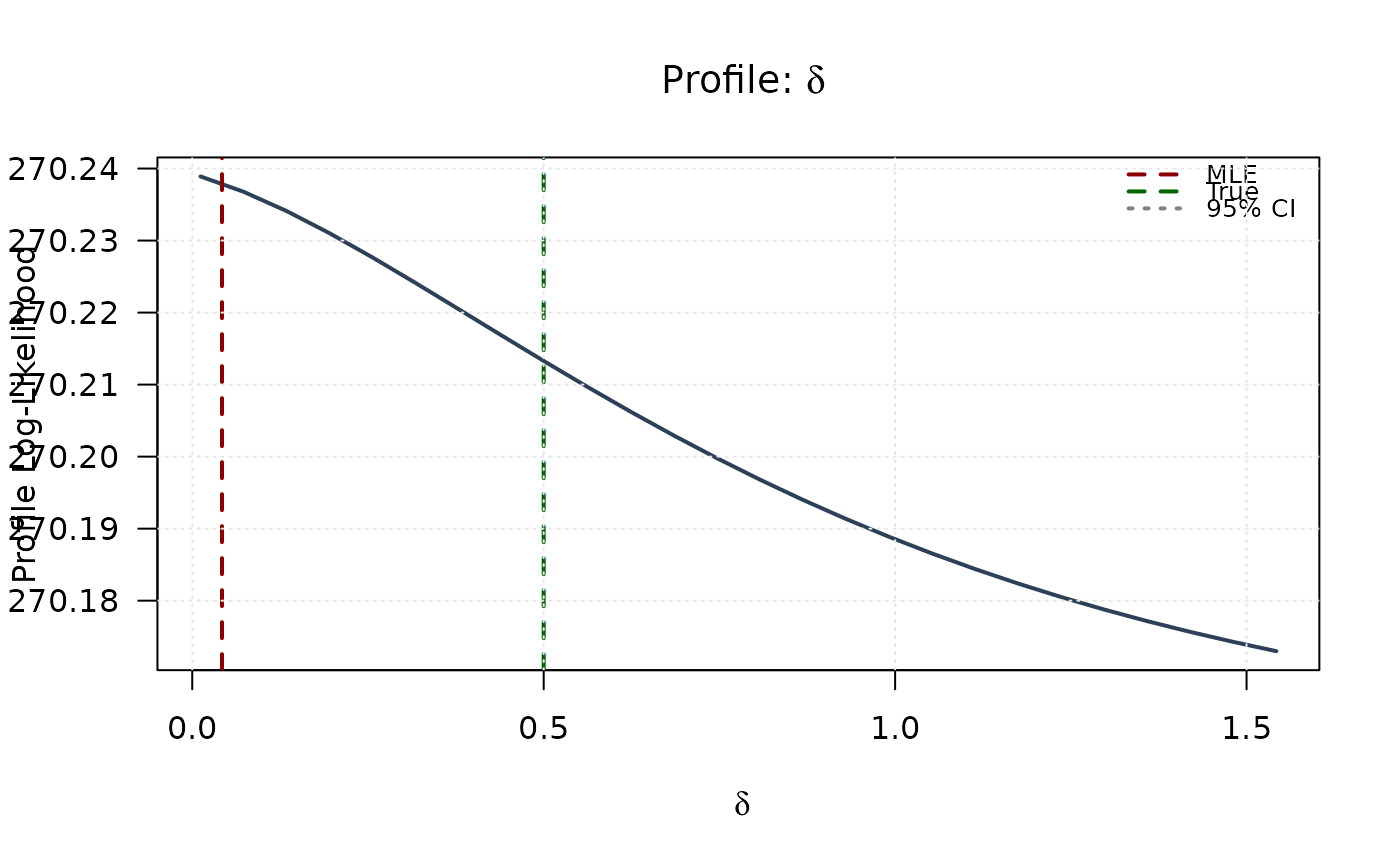
# Profile for delta
delta_grid <- seq(mle[4] - 1.5, mle[4] + 1.5, length.out = 50)
delta_grid <- delta_grid[delta_grid > 0]
profile_ll_delta <- numeric(length(delta_grid))
for (i in seq_along(delta_grid)) {
profile_fit <- optim(
par = mle[-4],
fn = function(p) llbkw(c(p[1], p[2], p[3], delta_grid[i]), data),
method = "Nelder-Mead"
)
profile_ll_delta[i] <- -profile_fit$value
}
# 95% confidence threshold
chi_crit <- qchisq(0.95, df = 1)
threshold <- max(profile_ll_alpha) - chi_crit / 2
# Plot all profiles
plot(alpha_grid, profile_ll_alpha,
type = "l", lwd = 2, col = "#2E4057",
xlab = expression(alpha), ylab = "Profile Log-Likelihood",
main = expression(paste("Profile: ", alpha)), las = 1
)
abline(v = mle[1], col = "#8B0000", lty = 2, lwd = 2)
abline(v = true_params[1], col = "#006400", lty = 2, lwd = 2)
abline(h = threshold, col = "#808080", lty = 3, lwd = 1.5)
legend("topright",
legend = c("MLE", "True", "95% CI"),
col = c("#8B0000", "#006400", "#808080"),
lty = c(2, 2, 3), lwd = 2, bty = "n", cex = 0.8
)
grid(col = "gray90")
 plot(beta_grid, profile_ll_beta,
type = "l", lwd = 2, col = "#2E4057",
xlab = expression(beta), ylab = "Profile Log-Likelihood",
main = expression(paste("Profile: ", beta)), las = 1
)
abline(v = mle[2], col = "#8B0000", lty = 2, lwd = 2)
abline(v = true_params[2], col = "#006400", lty = 2, lwd = 2)
abline(h = threshold, col = "#808080", lty = 3, lwd = 1.5)
legend("topright",
legend = c("MLE", "True", "95% CI"),
col = c("#8B0000", "#006400", "#808080"),
lty = c(2, 2, 3), lwd = 2, bty = "n", cex = 0.8
)
grid(col = "gray90")
plot(beta_grid, profile_ll_beta,
type = "l", lwd = 2, col = "#2E4057",
xlab = expression(beta), ylab = "Profile Log-Likelihood",
main = expression(paste("Profile: ", beta)), las = 1
)
abline(v = mle[2], col = "#8B0000", lty = 2, lwd = 2)
abline(v = true_params[2], col = "#006400", lty = 2, lwd = 2)
abline(h = threshold, col = "#808080", lty = 3, lwd = 1.5)
legend("topright",
legend = c("MLE", "True", "95% CI"),
col = c("#8B0000", "#006400", "#808080"),
lty = c(2, 2, 3), lwd = 2, bty = "n", cex = 0.8
)
grid(col = "gray90")
 plot(gamma_grid, profile_ll_gamma,
type = "l", lwd = 2, col = "#2E4057",
xlab = expression(gamma), ylab = "Profile Log-Likelihood",
main = expression(paste("Profile: ", gamma)), las = 1
)
abline(v = mle[3], col = "#8B0000", lty = 2, lwd = 2)
abline(v = true_params[3], col = "#006400", lty = 2, lwd = 2)
abline(h = threshold, col = "#808080", lty = 3, lwd = 1.5)
legend("topright",
legend = c("MLE", "True", "95% CI"),
col = c("#8B0000", "#006400", "#808080"),
lty = c(2, 2, 3), lwd = 2, bty = "n", cex = 0.8
)
grid(col = "gray90")
plot(gamma_grid, profile_ll_gamma,
type = "l", lwd = 2, col = "#2E4057",
xlab = expression(gamma), ylab = "Profile Log-Likelihood",
main = expression(paste("Profile: ", gamma)), las = 1
)
abline(v = mle[3], col = "#8B0000", lty = 2, lwd = 2)
abline(v = true_params[3], col = "#006400", lty = 2, lwd = 2)
abline(h = threshold, col = "#808080", lty = 3, lwd = 1.5)
legend("topright",
legend = c("MLE", "True", "95% CI"),
col = c("#8B0000", "#006400", "#808080"),
lty = c(2, 2, 3), lwd = 2, bty = "n", cex = 0.8
)
grid(col = "gray90")
 plot(delta_grid, profile_ll_delta,
type = "l", lwd = 2, col = "#2E4057",
xlab = expression(delta), ylab = "Profile Log-Likelihood",
main = expression(paste("Profile: ", delta)), las = 1
)
abline(v = mle[4], col = "#8B0000", lty = 2, lwd = 2)
abline(v = true_params[4], col = "#006400", lty = 2, lwd = 2)
abline(h = threshold, col = "#808080", lty = 3, lwd = 1.5)
legend("topright",
legend = c("MLE", "True", "95% CI"),
col = c("#8B0000", "#006400", "#808080"),
lty = c(2, 2, 3), lwd = 2, bty = "n", cex = 0.8
)
grid(col = "gray90")
plot(delta_grid, profile_ll_delta,
type = "l", lwd = 2, col = "#2E4057",
xlab = expression(delta), ylab = "Profile Log-Likelihood",
main = expression(paste("Profile: ", delta)), las = 1
)
abline(v = mle[4], col = "#8B0000", lty = 2, lwd = 2)
abline(v = true_params[4], col = "#006400", lty = 2, lwd = 2)
abline(h = threshold, col = "#808080", lty = 3, lwd = 1.5)
legend("topright",
legend = c("MLE", "True", "95% CI"),
col = c("#8B0000", "#006400", "#808080"),
lty = c(2, 2, 3), lwd = 2, bty = "n", cex = 0.8
)
grid(col = "gray90")
 ## Example 6: 2D Log-Likelihood Surfaces (Selected pairs)
# Create 2D grids with wider range (±1.5)
alpha_2d <- seq(mle[1] - 1.5, mle[1] + 1.5, length.out = round(n / 25))
beta_2d <- seq(mle[2] - 1.5, mle[2] + 1.5, length.out = round(n / 25))
gamma_2d <- seq(mle[3] - 1.5, mle[3] + 1.5, length.out = round(n / 25))
delta_2d <- seq(mle[4] - 1.5, mle[4] + 1.5, length.out = round(n / 25))
alpha_2d <- alpha_2d[alpha_2d > 0]
beta_2d <- beta_2d[beta_2d > 0]
gamma_2d <- gamma_2d[gamma_2d > 0]
delta_2d <- delta_2d[delta_2d > 0]
# Compute selected log-likelihood surfaces
ll_surface_ab <- matrix(NA, nrow = length(alpha_2d), ncol = length(beta_2d))
ll_surface_ag <- matrix(NA, nrow = length(alpha_2d), ncol = length(gamma_2d))
ll_surface_bd <- matrix(NA, nrow = length(beta_2d), ncol = length(delta_2d))
# Alpha vs Beta
for (i in seq_along(alpha_2d)) {
for (j in seq_along(beta_2d)) {
ll_surface_ab[i, j] <- -llbkw(c(alpha_2d[i], beta_2d[j], mle[3], mle[4]), data)
}
}
# Alpha vs Gamma
for (i in seq_along(alpha_2d)) {
for (j in seq_along(gamma_2d)) {
ll_surface_ag[i, j] <- -llbkw(c(alpha_2d[i], mle[2], gamma_2d[j], mle[4]), data)
}
}
# Beta vs Delta
for (i in seq_along(beta_2d)) {
for (j in seq_along(delta_2d)) {
ll_surface_bd[i, j] <- -llbkw(c(mle[1], beta_2d[i], mle[3], delta_2d[j]), data)
}
}
# Confidence region levels
max_ll_ab <- max(ll_surface_ab, na.rm = TRUE)
max_ll_ag <- max(ll_surface_ag, na.rm = TRUE)
max_ll_bd <- max(ll_surface_bd, na.rm = TRUE)
levels_95_ab <- max_ll_ab - qchisq(0.95, df = 2) / 2
levels_95_ag <- max_ll_ag - qchisq(0.95, df = 2) / 2
levels_95_bd <- max_ll_bd - qchisq(0.95, df = 2) / 2
# Plot selected surfaces
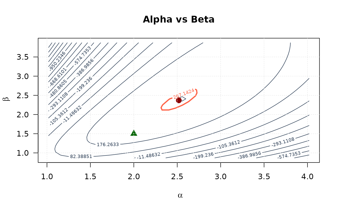
# Alpha vs Beta
contour(alpha_2d, beta_2d, ll_surface_ab,
xlab = expression(alpha), ylab = expression(beta),
main = "Alpha vs Beta", las = 1,
levels = seq(min(ll_surface_ab, na.rm = TRUE), max_ll_ab, length.out = 20),
col = "#2E4057", lwd = 1
)
contour(alpha_2d, beta_2d, ll_surface_ab,
levels = levels_95_ab, col = "#FF6347", lwd = 2.5, lty = 1, add = TRUE
)
points(mle[1], mle[2], pch = 19, col = "#8B0000", cex = 1.5)
points(true_params[1], true_params[2], pch = 17, col = "#006400", cex = 1.5)
grid(col = "gray90")
## Example 6: 2D Log-Likelihood Surfaces (Selected pairs)
# Create 2D grids with wider range (±1.5)
alpha_2d <- seq(mle[1] - 1.5, mle[1] + 1.5, length.out = round(n / 25))
beta_2d <- seq(mle[2] - 1.5, mle[2] + 1.5, length.out = round(n / 25))
gamma_2d <- seq(mle[3] - 1.5, mle[3] + 1.5, length.out = round(n / 25))
delta_2d <- seq(mle[4] - 1.5, mle[4] + 1.5, length.out = round(n / 25))
alpha_2d <- alpha_2d[alpha_2d > 0]
beta_2d <- beta_2d[beta_2d > 0]
gamma_2d <- gamma_2d[gamma_2d > 0]
delta_2d <- delta_2d[delta_2d > 0]
# Compute selected log-likelihood surfaces
ll_surface_ab <- matrix(NA, nrow = length(alpha_2d), ncol = length(beta_2d))
ll_surface_ag <- matrix(NA, nrow = length(alpha_2d), ncol = length(gamma_2d))
ll_surface_bd <- matrix(NA, nrow = length(beta_2d), ncol = length(delta_2d))
# Alpha vs Beta
for (i in seq_along(alpha_2d)) {
for (j in seq_along(beta_2d)) {
ll_surface_ab[i, j] <- -llbkw(c(alpha_2d[i], beta_2d[j], mle[3], mle[4]), data)
}
}
# Alpha vs Gamma
for (i in seq_along(alpha_2d)) {
for (j in seq_along(gamma_2d)) {
ll_surface_ag[i, j] <- -llbkw(c(alpha_2d[i], mle[2], gamma_2d[j], mle[4]), data)
}
}
# Beta vs Delta
for (i in seq_along(beta_2d)) {
for (j in seq_along(delta_2d)) {
ll_surface_bd[i, j] <- -llbkw(c(mle[1], beta_2d[i], mle[3], delta_2d[j]), data)
}
}
# Confidence region levels
max_ll_ab <- max(ll_surface_ab, na.rm = TRUE)
max_ll_ag <- max(ll_surface_ag, na.rm = TRUE)
max_ll_bd <- max(ll_surface_bd, na.rm = TRUE)
levels_95_ab <- max_ll_ab - qchisq(0.95, df = 2) / 2
levels_95_ag <- max_ll_ag - qchisq(0.95, df = 2) / 2
levels_95_bd <- max_ll_bd - qchisq(0.95, df = 2) / 2
# Plot selected surfaces
# Alpha vs Beta
contour(alpha_2d, beta_2d, ll_surface_ab,
xlab = expression(alpha), ylab = expression(beta),
main = "Alpha vs Beta", las = 1,
levels = seq(min(ll_surface_ab, na.rm = TRUE), max_ll_ab, length.out = 20),
col = "#2E4057", lwd = 1
)
contour(alpha_2d, beta_2d, ll_surface_ab,
levels = levels_95_ab, col = "#FF6347", lwd = 2.5, lty = 1, add = TRUE
)
points(mle[1], mle[2], pch = 19, col = "#8B0000", cex = 1.5)
points(true_params[1], true_params[2], pch = 17, col = "#006400", cex = 1.5)
grid(col = "gray90")
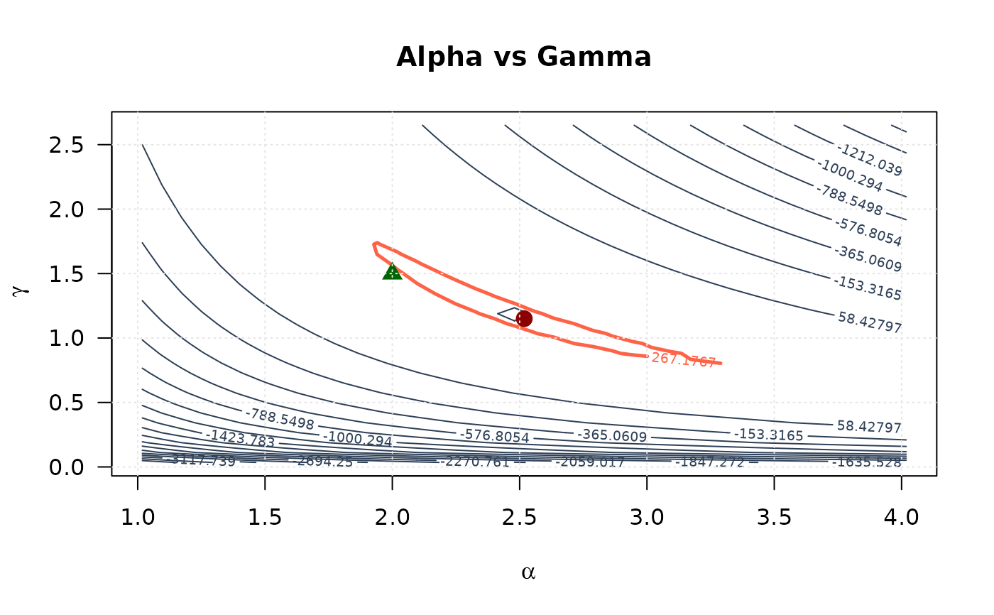
 # Alpha vs Gamma
contour(alpha_2d, gamma_2d, ll_surface_ag,
xlab = expression(alpha), ylab = expression(gamma),
main = "Alpha vs Gamma", las = 1,
levels = seq(min(ll_surface_ag, na.rm = TRUE), max_ll_ag, length.out = 20),
col = "#2E4057", lwd = 1
)
contour(alpha_2d, gamma_2d, ll_surface_ag,
levels = levels_95_ag, col = "#FF6347", lwd = 2.5, lty = 1, add = TRUE
)
points(mle[1], mle[3], pch = 19, col = "#8B0000", cex = 1.5)
points(true_params[1], true_params[3], pch = 17, col = "#006400", cex = 1.5)
grid(col = "gray90")
# Alpha vs Gamma
contour(alpha_2d, gamma_2d, ll_surface_ag,
xlab = expression(alpha), ylab = expression(gamma),
main = "Alpha vs Gamma", las = 1,
levels = seq(min(ll_surface_ag, na.rm = TRUE), max_ll_ag, length.out = 20),
col = "#2E4057", lwd = 1
)
contour(alpha_2d, gamma_2d, ll_surface_ag,
levels = levels_95_ag, col = "#FF6347", lwd = 2.5, lty = 1, add = TRUE
)
points(mle[1], mle[3], pch = 19, col = "#8B0000", cex = 1.5)
points(true_params[1], true_params[3], pch = 17, col = "#006400", cex = 1.5)
grid(col = "gray90")
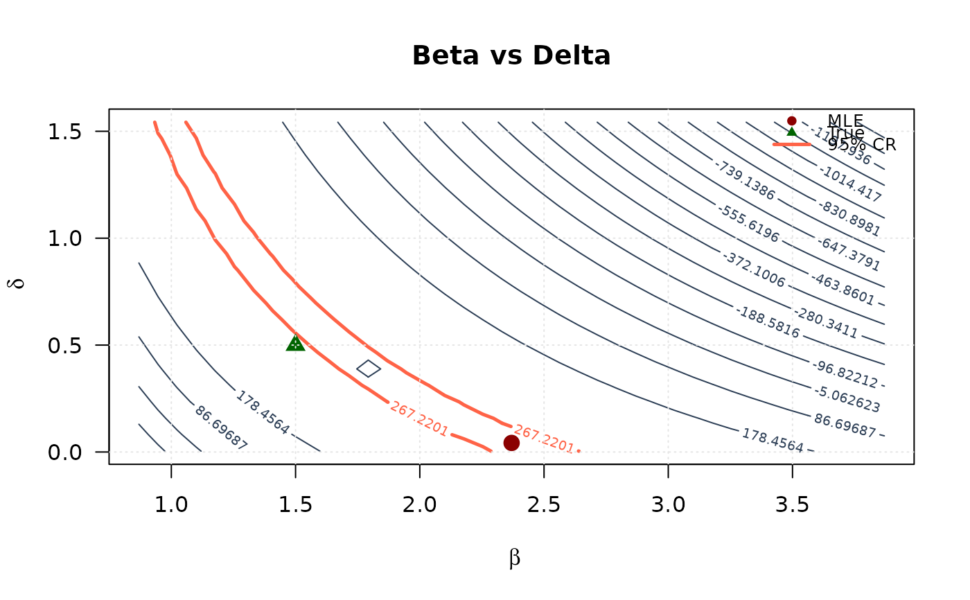
 # Beta vs Delta
contour(beta_2d, delta_2d, ll_surface_bd,
xlab = expression(beta), ylab = expression(delta),
main = "Beta vs Delta", las = 1,
levels = seq(min(ll_surface_bd, na.rm = TRUE), max_ll_bd, length.out = 20),
col = "#2E4057", lwd = 1
)
contour(beta_2d, delta_2d, ll_surface_bd,
levels = levels_95_bd, col = "#FF6347", lwd = 2.5, lty = 1, add = TRUE
)
points(mle[2], mle[4], pch = 19, col = "#8B0000", cex = 1.5)
points(true_params[2], true_params[4], pch = 17, col = "#006400", cex = 1.5)
grid(col = "gray90")
legend("topright",
legend = c("MLE", "True", "95% CR"),
col = c("#8B0000", "#006400", "#FF6347"),
pch = c(19, 17, NA),
lty = c(NA, NA, 1),
lwd = c(NA, NA, 2.5),
bty = "n", cex = 0.8
)
# Beta vs Delta
contour(beta_2d, delta_2d, ll_surface_bd,
xlab = expression(beta), ylab = expression(delta),
main = "Beta vs Delta", las = 1,
levels = seq(min(ll_surface_bd, na.rm = TRUE), max_ll_bd, length.out = 20),
col = "#2E4057", lwd = 1
)
contour(beta_2d, delta_2d, ll_surface_bd,
levels = levels_95_bd, col = "#FF6347", lwd = 2.5, lty = 1, add = TRUE
)
points(mle[2], mle[4], pch = 19, col = "#8B0000", cex = 1.5)
points(true_params[2], true_params[4], pch = 17, col = "#006400", cex = 1.5)
grid(col = "gray90")
legend("topright",
legend = c("MLE", "True", "95% CR"),
col = c("#8B0000", "#006400", "#FF6347"),
pch = c(19, 17, NA),
lty = c(NA, NA, 1),
lwd = c(NA, NA, 2.5),
bty = "n", cex = 0.8
)
 # }
# }