Cumulative Distribution Function (CDF) of the Beta-Kumaraswamy (BKw) Distribution

Computes the cumulative distribution function (CDF), $P(X \le q)$, for the Beta-Kumaraswamy (BKw) distribution with parameters alpha ($\alpha$), beta ($\beta$), gamma ($\gamma$), and delta ($\delta$). This distribution is defined on the interval (0, 1) and is a special case of the Generalized Kumaraswamy (GKw) distribution where $\lambda = 1$.

Usage

pbkw(q, alpha, beta, gamma, delta, lower_tail = TRUE, log_p = FALSE)

Arguments

q: Vector of quantiles (values generally between 0 and 1).
alpha: Shape parameter alpha > 0. Can be a scalar or a vector. Default: 1.0.
beta: Shape parameter beta > 0. Can be a scalar or a vector. Default: 1.0.
gamma: Shape parameter gamma > 0. Can be a scalar or a vector. Default: 1.0.
delta: Shape parameter delta >= 0. Can be a scalar or a vector. Default: 0.0.
lower_tail: Logical; if TRUE (default), probabilities are $P(X \le q)$, otherwise, $P(X > q)$.
log_p: Logical; if TRUE, probabilities $p$ are given as $\log(p)$. Default: FALSE.

Value

A vector of probabilities, $F(q)$, or their logarithms/complements depending on lower_tail and log_p. The length of the result is determined by the recycling rule applied to the arguments (q, alpha, beta, gamma, delta). Returns 0 (or -Inf if log_p = TRUE) for q <= 0 and 1 (or 0 if log_p = TRUE) for q >= 1. Returns NaN for invalid parameters.

Details

The Beta-Kumaraswamy (BKw) distribution is a special case of the five-parameter Generalized Kumaraswamy distribution (pgkw) obtained by setting the shape parameter $\lambda = 1$.

The CDF of the GKw distribution is $F_{GKw}(q) = I_{y(q)}(\gamma, \delta+1)$, where $y(q) = [1-(1-q^{\alpha})^{\beta}]^{\lambda}$ and $I_x(a,b)$ is the regularized incomplete beta function (pbeta). Setting $\lambda=1$ simplifies $y(q)$ to $1 - (1 - q^\alpha)^\beta$, yielding the BKw CDF: $$ F(q; \alpha, \beta, \gamma, \delta) = I_{1 - (1 - q^\alpha)^\beta}(\gamma, \delta+1) $$ This is evaluated using the pbeta function.

References

Cordeiro, G. M., & de Castro, M. (2011). A new family of generalized distributions. Journal of Statistical Computation and Simulation

Kumaraswamy, P. (1980). A generalized probability density function for double-bounded random processes. Journal of Hydrology, 46(1-2), 79-88.

Author

Lopes, J. E.

Examples

# \donttest{
# Example values
q_vals <- c(0.2, 0.5, 0.8)
alpha_par <- 2.0
beta_par <- 1.5
gamma_par <- 1.0
delta_par <- 0.5

# Calculate CDF P(X <= q)
probs <- pbkw(q_vals, alpha_par, beta_par, gamma_par, delta_par)
print(probs)
#> [1] 0.08775756 0.47653477 0.89961227

# Calculate upper tail P(X > q)
probs_upper <- pbkw(q_vals, alpha_par, beta_par, gamma_par, delta_par,
                    lower_tail = FALSE)
print(probs_upper)
#> [1] 0.9122424 0.5234652 0.1003877
# Check: probs + probs_upper should be 1
print(probs + probs_upper)
#> [1] 1 1 1

# Calculate log CDF
log_probs <- pbkw(q_vals, alpha_par, beta_par, gamma_par, delta_par,
                  log_p = TRUE)
print(log_probs)
#> [1] -2.4331773 -0.7412146 -0.1057914
# Check: should match log(probs)
print(log(probs))
#> [1] -2.4331773 -0.7412146 -0.1057914

# Compare with pgkw setting lambda = 1
probs_gkw <- pgkw(q_vals, alpha_par, beta_par, gamma = gamma_par,
                 delta = delta_par, lambda = 1.0)
print(paste("Max difference:", max(abs(probs - probs_gkw)))) # Should be near zero
#> [1] "Max difference: 0"

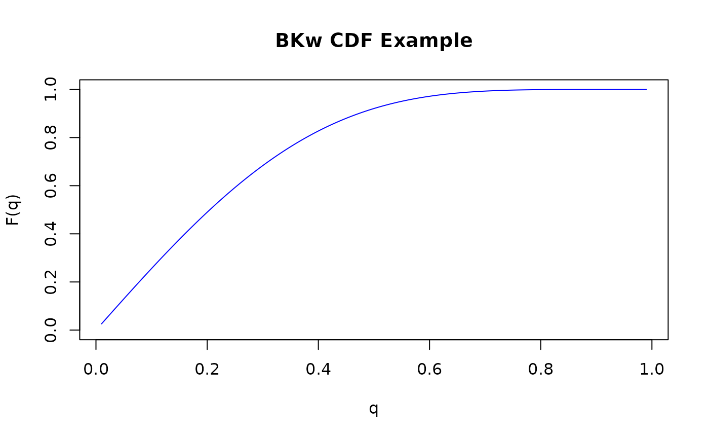
# Plot the CDF
curve_q <- seq(0.01, 0.99, length.out = 200)
curve_p <- pbkw(curve_q, alpha = 2, beta = 3, gamma = 0.5, delta = 1)
plot(curve_q, curve_p, type = "l", main = "BKw CDF Example",
     xlab = "q", ylab = "F(q)", col = "blue", ylim = c(0, 1))

# }