Density of the Beta-Kumaraswamy (BKw) Distribution

Computes the probability density function (PDF) for the Beta-Kumaraswamy (BKw) distribution with parameters alpha ($\alpha$), beta ($\beta$), gamma ($\gamma$), and delta ($\delta$). This distribution is defined on the interval (0, 1).

Usage

dbkw(x, alpha, beta, gamma, delta, log_prob = FALSE)

Arguments

x: Vector of quantiles (values between 0 and 1).
alpha: Shape parameter alpha > 0. Can be a scalar or a vector. Default: 1.0.
beta: Shape parameter beta > 0. Can be a scalar or a vector. Default: 1.0.
gamma: Shape parameter gamma > 0. Can be a scalar or a vector. Default: 1.0.
delta: Shape parameter delta >= 0. Can be a scalar or a vector. Default: 0.0.
log_prob: Logical; if TRUE, the logarithm of the density is returned ($\log(f(x))$). Default: FALSE.

Value

A vector of density values ($f(x)$) or log-density values ($\log(f(x))$). The length of the result is determined by the recycling rule applied to the arguments (x, alpha, beta, gamma, delta). Returns 0 (or -Inf if log_prob = TRUE) for x outside the interval (0, 1), or NaN if parameters are invalid (e.g., alpha <= 0, beta <= 0, gamma <= 0, delta < 0).

Details

The probability density function (PDF) of the Beta-Kumaraswamy (BKw) distribution is given by: $$ f(x; \alpha, \beta, \gamma, \delta) = \frac{\alpha \beta}{B(\gamma, \delta+1)} x^{\alpha - 1} \bigl(1 - x^\alpha\bigr)^{\beta(\delta+1) - 1} \bigl[1 - \bigl(1 - x^\alpha\bigr)^\beta\bigr]^{\gamma - 1} $$ for $0 < x < 1$, where $B(a,b)$ is the Beta function (beta).

The BKw distribution is a special case of the five-parameter Generalized Kumaraswamy (GKw) distribution (dgkw) obtained by setting the parameter $\lambda = 1$. Numerical evaluation is performed using algorithms similar to those for dgkw, ensuring stability.

References

Cordeiro, G. M., & de Castro, M. (2011). A new family of generalized distributions. Journal of Statistical Computation and Simulation

Kumaraswamy, P. (1980). A generalized probability density function for double-bounded random processes. Journal of Hydrology, 46(1-2), 79-88.

Author

Lopes, J. E.

Examples

# \donttest{
# Example values
x_vals <- c(0.2, 0.5, 0.8)
alpha_par <- 2.0
beta_par <- 1.5
gamma_par <- 1.0 # Equivalent to Kw when gamma=1
delta_par <- 0.5

# Calculate density
densities <- dbkw(x_vals, alpha_par, beta_par, gamma_par, delta_par)
print(densities)
#> [1] 0.8552273 1.5703957 1.0038773

# Calculate log-density
log_densities <- dbkw(x_vals, alpha_par, beta_par, gamma_par, delta_par,
                      log_prob = TRUE)
print(log_densities)
#> [1] -0.156388009  0.451327626  0.003869786
# Check: should match log(densities)
print(log(densities))
#> [1] -0.156388009  0.451327626  0.003869786

# Compare with dgkw setting lambda = 1
densities_gkw <- dgkw(x_vals, alpha_par, beta_par, gamma = gamma_par,
                      delta = delta_par, lambda = 1.0)
print(paste("Max difference:", max(abs(densities - densities_gkw)))) # Should be near zero
#> [1] "Max difference: 2.22044604925031e-16"

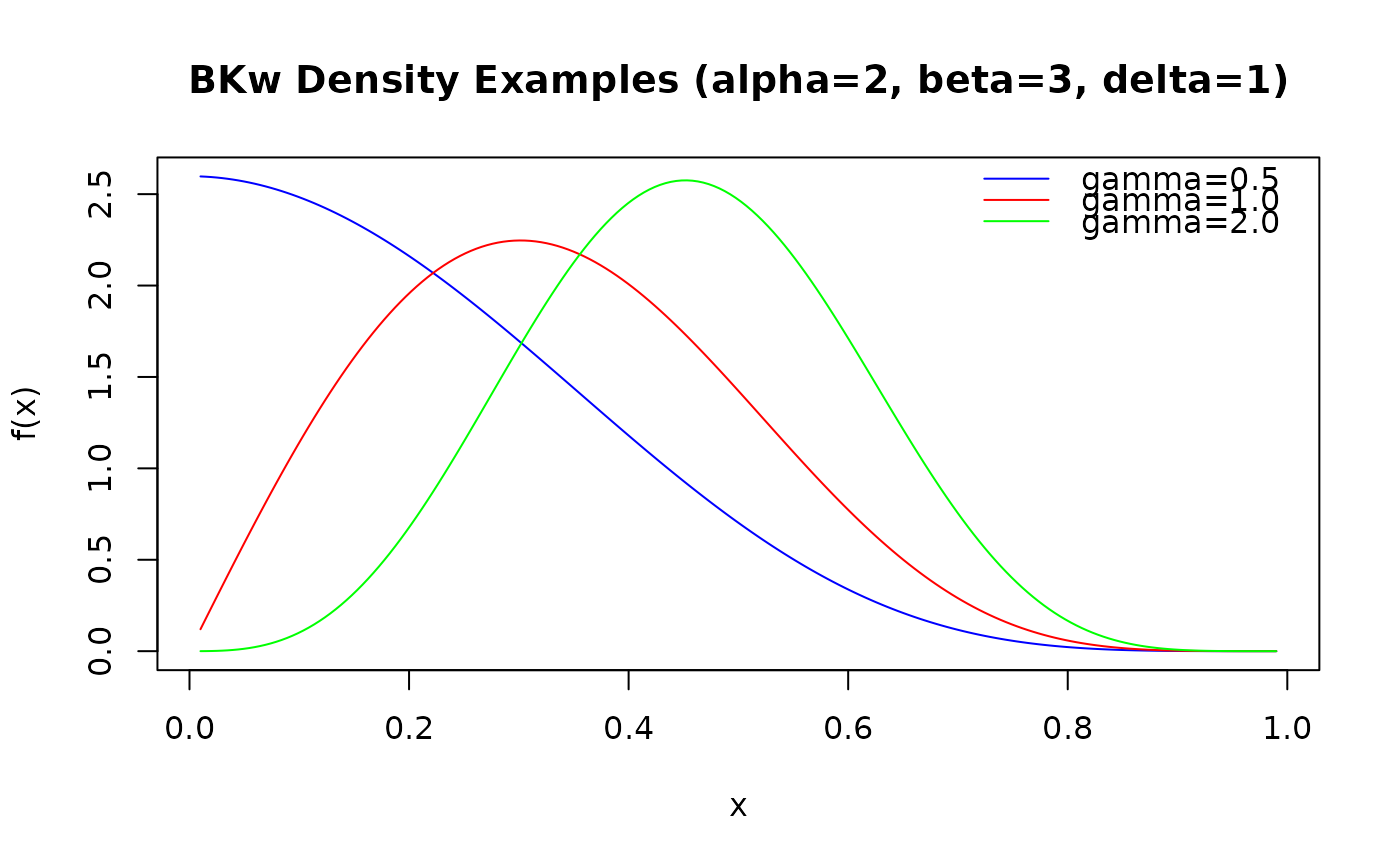
# Plot the density for different gamma values
curve_x <- seq(0.01, 0.99, length.out = 200)
curve_y1 <- dbkw(curve_x, alpha = 2, beta = 3, gamma = 0.5, delta = 1)
curve_y2 <- dbkw(curve_x, alpha = 2, beta = 3, gamma = 1.0, delta = 1)
curve_y3 <- dbkw(curve_x, alpha = 2, beta = 3, gamma = 2.0, delta = 1)

plot(curve_x, curve_y1, type = "l", main = "BKw Density Examples (alpha=2, beta=3, delta=1)",
     xlab = "x", ylab = "f(x)", col = "blue", ylim = range(0, curve_y1, curve_y2, curve_y3))
lines(curve_x, curve_y2, col = "red")
lines(curve_x, curve_y3, col = "green")
legend("topright", legend = c("gamma=0.5", "gamma=1.0", "gamma=2.0"),
       col = c("blue", "red", "green"), lty = 1, bty = "n")

# }