Computes the negative log-likelihood function for the five-parameter Generalized Kumaraswamy (GKw) distribution given a vector of observations. This function is designed for use in optimization routines (e.g., maximum likelihood estimation).
Arguments
- par
A numeric vector of length 5 containing the distribution parameters in the order:
alpha(\(\alpha > 0\)),beta(\(\beta > 0\)),gamma(\(\gamma > 0\)),delta(\(\delta \ge 0\)),lambda(\(\lambda > 0\)).- data
A numeric vector of observations. All values must be strictly between 0 and 1 (exclusive).
Value
Returns a single double value representing the negative
log-likelihood (\(-\ell(\theta|\mathbf{x})\)). Returns a large positive
value (e.g., Inf) if any parameter values in par are invalid
according to their constraints, or if any value in data is not in
the interval (0, 1).
Details
The probability density function (PDF) of the GKw distribution is given in
dgkw. The log-likelihood function \(\ell(\theta)\) for a sample
\(\mathbf{x} = (x_1, \dots, x_n)\) is:
$$
\ell(\theta | \mathbf{x}) = n\ln(\lambda\alpha\beta) - n\ln B(\gamma,\delta+1) +
\sum_{i=1}^{n} [(\alpha-1)\ln(x_i) + (\beta-1)\ln(v_i) + (\gamma\lambda-1)\ln(w_i) + \delta\ln(z_i)]
$$
where \(\theta = (\alpha, \beta, \gamma, \delta, \lambda)\), \(B(a,b)\)
is the Beta function (beta), and:
\(v_i = 1 - x_i^{\alpha}\)
\(w_i = 1 - v_i^{\beta} = 1 - (1-x_i^{\alpha})^{\beta}\)
\(z_i = 1 - w_i^{\lambda} = 1 - [1-(1-x_i^{\alpha})^{\beta}]^{\lambda}\)
This function computes \(-\ell(\theta|\mathbf{x})\).
Numerical stability is prioritized using:
References
Cordeiro, G. M., & de Castro, M. (2011). A new family of generalized distributions. Journal of Statistical Computation and Simulation
Kumaraswamy, P. (1980). A generalized probability density function for double-bounded random processes. Journal of Hydrology, 46(1-2), 79-88.
Examples
# \donttest{
## Example 1: Basic Log-Likelihood Evaluation
# Generate sample data
set.seed(123)
n <- 1000
true_params <- c(alpha = 2.0, beta = 3.0, gamma = 1.5, delta = 2.0, lambda = 1.8)
data <- rgkw(n,
alpha = true_params[1], beta = true_params[2],
gamma = true_params[3], delta = true_params[4],
lambda = true_params[5]
)
# Evaluate negative log-likelihood at true parameters
nll_true <- llgkw(par = true_params, data = data)
cat("Negative log-likelihood at true parameters:", nll_true, "\n")
#> Negative log-likelihood at true parameters: -703.5634
# Evaluate at different parameter values
test_params <- rbind(
c(1.5, 2.5, 1.2, 1.5, 1.5),
c(2.0, 3.0, 1.5, 2.0, 1.8),
c(2.5, 3.5, 1.8, 2.5, 2.0)
)
nll_values <- apply(test_params, 1, function(p) llgkw(p, data))
results <- data.frame(
Alpha = test_params[, 1],
Beta = test_params[, 2],
Gamma = test_params[, 3],
Delta = test_params[, 4],
Lambda = test_params[, 5],
NegLogLik = nll_values
)
print(results, digits = 4)
#> Alpha Beta Gamma Delta Lambda NegLogLik
#> 1 1.5 2.5 1.2 1.5 1.5 -376.1
#> 2 2.0 3.0 1.5 2.0 1.8 -703.6
#> 3 2.5 3.5 1.8 2.5 2.0 -425.3
## Example 2: Maximum Likelihood Estimation
# Optimization using BFGS with analytical gradient
fit <- optim(
par = c(1.5, 2.5, 1.2, 1.5, 1.5),
fn = llgkw,
gr = grgkw,
data = data,
method = "BFGS",
hessian = TRUE,
control = list(maxit = 1000)
)
mle <- fit$par
names(mle) <- c("alpha", "beta", "gamma", "delta", "lambda")
se <- sqrt(diag(solve(fit$hessian)))
results <- data.frame(
Parameter = c("alpha", "beta", "gamma", "delta", "lambda"),
True = true_params,
MLE = mle,
SE = se,
CI_Lower = mle - 1.96 * se,
CI_Upper = mle + 1.96 * se
)
print(results, digits = 4)
#> Parameter True MLE SE CI_Lower CI_Upper
#> alpha alpha 2.0 1.0702 1.8188 -2.4946 4.635
#> beta beta 3.0 3.0748 3.3714 -3.5332 9.683
#> gamma gamma 1.5 0.3822 0.3844 -0.3714 1.136
#> delta delta 2.0 1.6150 2.7406 -3.7565 6.987
#> lambda lambda 1.8 16.2353 30.0703 -42.7024 75.173
cat("\nNegative log-likelihood at MLE:", fit$value, "\n")
#>
#> Negative log-likelihood at MLE: -704.3541
cat("AIC:", 2 * fit$value + 2 * length(mle), "\n")
#> AIC: -1398.708
cat("BIC:", 2 * fit$value + length(mle) * log(n), "\n")
#> BIC: -1374.17
## Example 3: Comparing Optimization Methods
methods <- c("BFGS", "Nelder-Mead")
start_params <- c(1.5, 2.5, 1.2, 1.5, 1.5)
comparison <- data.frame(
Method = character(),
Alpha = numeric(),
Beta = numeric(),
Gamma = numeric(),
Delta = numeric(),
Lambda = numeric(),
NegLogLik = numeric(),
Convergence = integer(),
stringsAsFactors = FALSE
)
for (method in methods) {
if (method == "BFGS") {
fit_temp <- optim(
par = start_params,
fn = llgkw,
gr = grgkw,
data = data,
method = method,
control = list(maxit = 1000)
)
} else if (method == "L-BFGS-B") {
fit_temp <- optim(
par = start_params,
fn = llgkw,
gr = grgkw,
data = data,
method = method,
lower = rep(0.001, 5),
upper = rep(20, 5),
control = list(maxit = 1000)
)
} else {
fit_temp <- optim(
par = start_params,
fn = llgkw,
data = data,
method = method,
control = list(maxit = 1000)
)
}
comparison <- rbind(comparison, data.frame(
Method = method,
Alpha = fit_temp$par[1],
Beta = fit_temp$par[2],
Gamma = fit_temp$par[3],
Delta = fit_temp$par[4],
Lambda = fit_temp$par[5],
NegLogLik = fit_temp$value,
Convergence = fit_temp$convergence,
stringsAsFactors = FALSE
))
}
print(comparison, digits = 4, row.names = FALSE)
#> Method Alpha Beta Gamma Delta Lambda NegLogLik Convergence
#> BFGS 1.070 3.075 0.3822 1.615 16.235 -704.4 0
#> Nelder-Mead 1.868 3.136 1.0095 1.870 2.826 -704.0 0
## Example 4: Likelihood Ratio Test
# Test H0: gamma = 1.5 vs H1: gamma free
loglik_full <- -fit$value
restricted_ll <- function(params_restricted, data, gamma_fixed) {
llgkw(
par = c(
params_restricted[1], params_restricted[2],
gamma_fixed, params_restricted[3], params_restricted[4]
),
data = data
)
}
fit_restricted <- optim(
par = c(mle[1], mle[2], mle[4], mle[5]),
fn = restricted_ll,
data = data,
gamma_fixed = 1.5,
method = "Nelder-Mead",
control = list(maxit = 1000)
)
loglik_restricted <- -fit_restricted$value
lr_stat <- 2 * (loglik_full - loglik_restricted)
p_value <- pchisq(lr_stat, df = 1, lower.tail = FALSE)
cat("LR Statistic:", round(lr_stat, 4), "\n")
#> LR Statistic: 0.8112
cat("P-value:", format.pval(p_value, digits = 4), "\n")
#> P-value: 0.3678
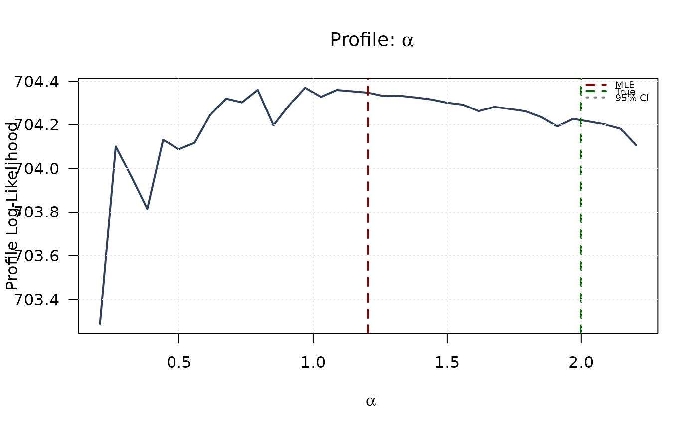
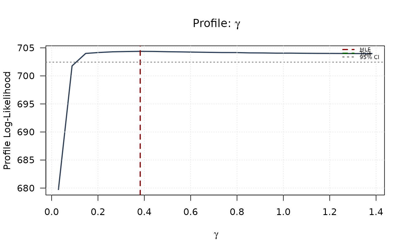
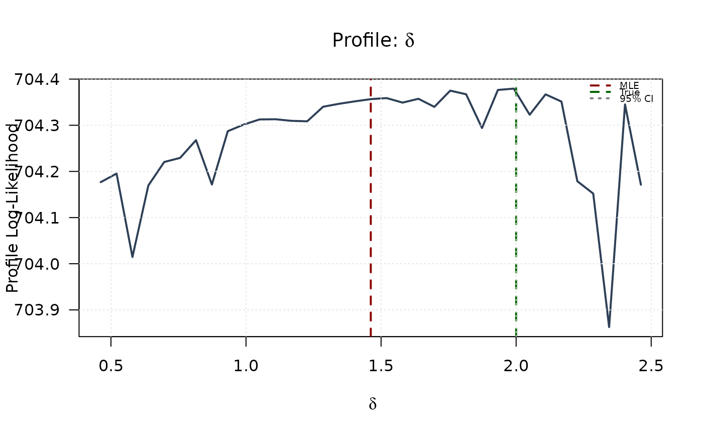
## Example 5: Univariate Profile Likelihoods
# Profile for alpha
xd <- 1
alpha_grid <- seq(mle[1] - xd, mle[1] + xd, length.out = 35)
alpha_grid <- alpha_grid[alpha_grid > 0]
profile_ll_alpha <- numeric(length(alpha_grid))
for (i in seq_along(alpha_grid)) {
profile_fit <- optim(
par = mle[-1],
fn = function(p) llgkw(c(alpha_grid[i], p), data),
method = "Nelder-Mead",
control = list(maxit = 500)
)
profile_ll_alpha[i] <- -profile_fit$value
}
# Profile for beta
beta_grid <- seq(mle[2] - xd, mle[2] + xd, length.out = 35)
beta_grid <- beta_grid[beta_grid > 0]
profile_ll_beta <- numeric(length(beta_grid))
for (i in seq_along(beta_grid)) {
profile_fit <- optim(
par = mle[-2],
fn = function(p) llgkw(c(p[1], beta_grid[i], p[2], p[3], p[4]), data),
method = "Nelder-Mead",
control = list(maxit = 500)
)
profile_ll_beta[i] <- -profile_fit$value
}
# Profile for gamma
gamma_grid <- seq(mle[3] - xd, mle[3] + xd, length.out = 35)
gamma_grid <- gamma_grid[gamma_grid > 0]
profile_ll_gamma <- numeric(length(gamma_grid))
for (i in seq_along(gamma_grid)) {
profile_fit <- optim(
par = mle[-3],
fn = function(p) llgkw(c(p[1], p[2], gamma_grid[i], p[3], p[4]), data),
method = "Nelder-Mead",
control = list(maxit = 500)
)
profile_ll_gamma[i] <- -profile_fit$value
}
# Profile for delta
delta_grid <- seq(mle[4] - xd, mle[4] + xd, length.out = 35)
delta_grid <- delta_grid[delta_grid > 0]
profile_ll_delta <- numeric(length(delta_grid))
for (i in seq_along(delta_grid)) {
profile_fit <- optim(
par = mle[-4],
fn = function(p) llgkw(c(p[1], p[2], p[3], delta_grid[i], p[4]), data),
method = "Nelder-Mead",
control = list(maxit = 500)
)
profile_ll_delta[i] <- -profile_fit$value
}
# Profile for lambda
lambda_grid <- seq(mle[5] - xd, mle[5] + xd, length.out = 35)
lambda_grid <- lambda_grid[lambda_grid > 0]
profile_ll_lambda <- numeric(length(lambda_grid))
for (i in seq_along(lambda_grid)) {
profile_fit <- optim(
par = mle[-5],
fn = function(p) llgkw(c(p[1], p[2], p[3], p[4], lambda_grid[i]), data),
method = "Nelder-Mead",
control = list(maxit = 500)
)
profile_ll_lambda[i] <- -profile_fit$value
}
# 95% confidence threshold
chi_crit <- qchisq(0.95, df = 1)
threshold <- max(profile_ll_alpha) - chi_crit / 2
# Plot all profiles
plot(alpha_grid, profile_ll_alpha,
type = "l", lwd = 2, col = "#2E4057",
xlab = expression(alpha), ylab = "Profile Log-Likelihood",
main = expression(paste("Profile: ", alpha)), las = 1
)
abline(v = mle[1], col = "#8B0000", lty = 2, lwd = 2)
abline(v = true_params[1], col = "#006400", lty = 2, lwd = 2)
abline(h = threshold, col = "#808080", lty = 3, lwd = 1.5)
legend("topright",
legend = c("MLE", "True", "95% CI"),
col = c("#8B0000", "#006400", "#808080"),
lty = c(2, 2, 3), lwd = 2, bty = "n", cex = 0.6
)
grid(col = "gray90")
 plot(beta_grid, profile_ll_beta,
type = "l", lwd = 2, col = "#2E4057",
xlab = expression(beta), ylab = "Profile Log-Likelihood",
main = expression(paste("Profile: ", beta)), las = 1
)
abline(v = mle[2], col = "#8B0000", lty = 2, lwd = 2)
abline(v = true_params[2], col = "#006400", lty = 2, lwd = 2)
abline(h = threshold, col = "#808080", lty = 3, lwd = 1.5)
legend("topright",
legend = c("MLE", "True", "95% CI"),
col = c("#8B0000", "#006400", "#808080"),
lty = c(2, 2, 3), lwd = 2, bty = "n", cex = 0.6
)
grid(col = "gray90")
plot(beta_grid, profile_ll_beta,
type = "l", lwd = 2, col = "#2E4057",
xlab = expression(beta), ylab = "Profile Log-Likelihood",
main = expression(paste("Profile: ", beta)), las = 1
)
abline(v = mle[2], col = "#8B0000", lty = 2, lwd = 2)
abline(v = true_params[2], col = "#006400", lty = 2, lwd = 2)
abline(h = threshold, col = "#808080", lty = 3, lwd = 1.5)
legend("topright",
legend = c("MLE", "True", "95% CI"),
col = c("#8B0000", "#006400", "#808080"),
lty = c(2, 2, 3), lwd = 2, bty = "n", cex = 0.6
)
grid(col = "gray90")
 plot(gamma_grid, profile_ll_gamma,
type = "l", lwd = 2, col = "#2E4057",
xlab = expression(gamma), ylab = "Profile Log-Likelihood",
main = expression(paste("Profile: ", gamma)), las = 1
)
abline(v = mle[3], col = "#8B0000", lty = 2, lwd = 2)
abline(v = true_params[3], col = "#006400", lty = 2, lwd = 2)
abline(h = threshold, col = "#808080", lty = 3, lwd = 1.5)
legend("topright",
legend = c("MLE", "True", "95% CI"),
col = c("#8B0000", "#006400", "#808080"),
lty = c(2, 2, 3), lwd = 2, bty = "n", cex = 0.6
)
grid(col = "gray90")
plot(gamma_grid, profile_ll_gamma,
type = "l", lwd = 2, col = "#2E4057",
xlab = expression(gamma), ylab = "Profile Log-Likelihood",
main = expression(paste("Profile: ", gamma)), las = 1
)
abline(v = mle[3], col = "#8B0000", lty = 2, lwd = 2)
abline(v = true_params[3], col = "#006400", lty = 2, lwd = 2)
abline(h = threshold, col = "#808080", lty = 3, lwd = 1.5)
legend("topright",
legend = c("MLE", "True", "95% CI"),
col = c("#8B0000", "#006400", "#808080"),
lty = c(2, 2, 3), lwd = 2, bty = "n", cex = 0.6
)
grid(col = "gray90")
 plot(delta_grid, profile_ll_delta,
type = "l", lwd = 2, col = "#2E4057",
xlab = expression(delta), ylab = "Profile Log-Likelihood",
main = expression(paste("Profile: ", delta)), las = 1
)
abline(v = mle[4], col = "#8B0000", lty = 2, lwd = 2)
abline(v = true_params[4], col = "#006400", lty = 2, lwd = 2)
abline(h = threshold, col = "#808080", lty = 3, lwd = 1.5)
legend("topright",
legend = c("MLE", "True", "95% CI"),
col = c("#8B0000", "#006400", "#808080"),
lty = c(2, 2, 3), lwd = 2, bty = "n", cex = 0.6
)
grid(col = "gray90")
plot(delta_grid, profile_ll_delta,
type = "l", lwd = 2, col = "#2E4057",
xlab = expression(delta), ylab = "Profile Log-Likelihood",
main = expression(paste("Profile: ", delta)), las = 1
)
abline(v = mle[4], col = "#8B0000", lty = 2, lwd = 2)
abline(v = true_params[4], col = "#006400", lty = 2, lwd = 2)
abline(h = threshold, col = "#808080", lty = 3, lwd = 1.5)
legend("topright",
legend = c("MLE", "True", "95% CI"),
col = c("#8B0000", "#006400", "#808080"),
lty = c(2, 2, 3), lwd = 2, bty = "n", cex = 0.6
)
grid(col = "gray90")
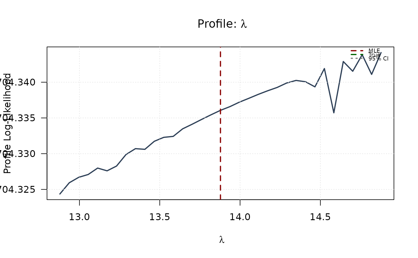
 plot(lambda_grid, profile_ll_lambda,
type = "l", lwd = 2, col = "#2E4057",
xlab = expression(lambda), ylab = "Profile Log-Likelihood",
main = expression(paste("Profile: ", lambda)), las = 1
)
abline(v = mle[5], col = "#8B0000", lty = 2, lwd = 2)
abline(v = true_params[5], col = "#006400", lty = 2, lwd = 2)
abline(h = threshold, col = "#808080", lty = 3, lwd = 1.5)
legend("topright",
legend = c("MLE", "True", "95% CI"),
col = c("#8B0000", "#006400", "#808080"),
lty = c(2, 2, 3), lwd = 2, bty = "n", cex = 0.6
)
grid(col = "gray90")
plot(lambda_grid, profile_ll_lambda,
type = "l", lwd = 2, col = "#2E4057",
xlab = expression(lambda), ylab = "Profile Log-Likelihood",
main = expression(paste("Profile: ", lambda)), las = 1
)
abline(v = mle[5], col = "#8B0000", lty = 2, lwd = 2)
abline(v = true_params[5], col = "#006400", lty = 2, lwd = 2)
abline(h = threshold, col = "#808080", lty = 3, lwd = 1.5)
legend("topright",
legend = c("MLE", "True", "95% CI"),
col = c("#8B0000", "#006400", "#808080"),
lty = c(2, 2, 3), lwd = 2, bty = "n", cex = 0.6
)
grid(col = "gray90")
 ## Example 6: 2D Log-Likelihood Surface (Alpha vs Beta)
# Plot all profiles
# Create 2D grid
alpha_2d <- seq(mle[1] - xd, mle[1] + xd, length.out = round(n / 4))
beta_2d <- seq(mle[2] - xd, mle[2] + xd, length.out = round(n / 4))
alpha_2d <- alpha_2d[alpha_2d > 0]
beta_2d <- beta_2d[beta_2d > 0]
# Compute log-likelihood surface
ll_surface_ab <- matrix(NA, nrow = length(alpha_2d), ncol = length(beta_2d))
for (i in seq_along(alpha_2d)) {
for (j in seq_along(beta_2d)) {
ll_surface_ab[i, j] <- llgkw(c(
alpha_2d[i], beta_2d[j],
mle[3], mle[4], mle[5]
), data)
}
}
# Confidence region levels
max_ll_ab <- max(ll_surface_ab, na.rm = TRUE)
levels_90_ab <- max_ll_ab - qchisq(0.90, df = 2) / 2
levels_95_ab <- max_ll_ab - qchisq(0.95, df = 2) / 2
levels_99_ab <- max_ll_ab - qchisq(0.99, df = 2) / 2
# Plot contour
contour(alpha_2d, beta_2d, ll_surface_ab,
xlab = expression(alpha), ylab = expression(beta),
main = "2D Log-Likelihood: Alpha vs Beta",
levels = seq(min(ll_surface_ab, na.rm = TRUE), max_ll_ab, length.out = 20),
col = "#2E4057", las = 1, lwd = 1
)
contour(alpha_2d, beta_2d, ll_surface_ab,
levels = c(levels_90_ab, levels_95_ab, levels_99_ab),
col = c("#FFA07A", "#FF6347", "#8B0000"),
lwd = c(2, 2.5, 3), lty = c(3, 2, 1),
add = TRUE, labcex = 0.8
)
points(mle[1], mle[2], pch = 19, col = "#8B0000", cex = 1.5)
points(true_params[1], true_params[2], pch = 17, col = "#006400", cex = 1.5)
legend("topright",
legend = c("MLE", "True", "90% CR", "95% CR", "99% CR"),
col = c("#8B0000", "#006400", "#FFA07A", "#FF6347", "#8B0000"),
pch = c(19, 17, NA, NA, NA),
lty = c(NA, NA, 3, 2, 1),
lwd = c(NA, NA, 2, 2.5, 3),
bty = "n", cex = 0.8
)
grid(col = "gray90")
## Example 6: 2D Log-Likelihood Surface (Alpha vs Beta)
# Plot all profiles
# Create 2D grid
alpha_2d <- seq(mle[1] - xd, mle[1] + xd, length.out = round(n / 4))
beta_2d <- seq(mle[2] - xd, mle[2] + xd, length.out = round(n / 4))
alpha_2d <- alpha_2d[alpha_2d > 0]
beta_2d <- beta_2d[beta_2d > 0]
# Compute log-likelihood surface
ll_surface_ab <- matrix(NA, nrow = length(alpha_2d), ncol = length(beta_2d))
for (i in seq_along(alpha_2d)) {
for (j in seq_along(beta_2d)) {
ll_surface_ab[i, j] <- llgkw(c(
alpha_2d[i], beta_2d[j],
mle[3], mle[4], mle[5]
), data)
}
}
# Confidence region levels
max_ll_ab <- max(ll_surface_ab, na.rm = TRUE)
levels_90_ab <- max_ll_ab - qchisq(0.90, df = 2) / 2
levels_95_ab <- max_ll_ab - qchisq(0.95, df = 2) / 2
levels_99_ab <- max_ll_ab - qchisq(0.99, df = 2) / 2
# Plot contour
contour(alpha_2d, beta_2d, ll_surface_ab,
xlab = expression(alpha), ylab = expression(beta),
main = "2D Log-Likelihood: Alpha vs Beta",
levels = seq(min(ll_surface_ab, na.rm = TRUE), max_ll_ab, length.out = 20),
col = "#2E4057", las = 1, lwd = 1
)
contour(alpha_2d, beta_2d, ll_surface_ab,
levels = c(levels_90_ab, levels_95_ab, levels_99_ab),
col = c("#FFA07A", "#FF6347", "#8B0000"),
lwd = c(2, 2.5, 3), lty = c(3, 2, 1),
add = TRUE, labcex = 0.8
)
points(mle[1], mle[2], pch = 19, col = "#8B0000", cex = 1.5)
points(true_params[1], true_params[2], pch = 17, col = "#006400", cex = 1.5)
legend("topright",
legend = c("MLE", "True", "90% CR", "95% CR", "99% CR"),
col = c("#8B0000", "#006400", "#FFA07A", "#FF6347", "#8B0000"),
pch = c(19, 17, NA, NA, NA),
lty = c(NA, NA, 3, 2, 1),
lwd = c(NA, NA, 2, 2.5, 3),
bty = "n", cex = 0.8
)
grid(col = "gray90")
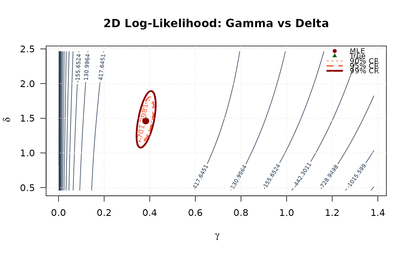
 ## Example 7: 2D Log-Likelihood Surface (Gamma vs Delta)
# Create 2D grid
gamma_2d <- seq(mle[3] - xd, mle[3] + xd, length.out = round(n / 4))
delta_2d <- seq(mle[4] - xd, mle[4] + xd, length.out = round(n / 4))
gamma_2d <- gamma_2d[gamma_2d > 0]
delta_2d <- delta_2d[delta_2d > 0]
# Compute log-likelihood surface
ll_surface_gd <- matrix(NA, nrow = length(gamma_2d), ncol = length(delta_2d))
for (i in seq_along(gamma_2d)) {
for (j in seq_along(delta_2d)) {
ll_surface_gd[i, j] <- -llgkw(c(
mle[1], mle[2], gamma_2d[i],
delta_2d[j], mle[5]
), data)
}
}
# Confidence region levels
max_ll_gd <- max(ll_surface_gd, na.rm = TRUE)
levels_90_gd <- max_ll_gd - qchisq(0.90, df = 2) / 2
levels_95_gd <- max_ll_gd - qchisq(0.95, df = 2) / 2
levels_99_gd <- max_ll_gd - qchisq(0.99, df = 2) / 2
# Plot contour
contour(gamma_2d, delta_2d, ll_surface_gd,
xlab = expression(gamma), ylab = expression(delta),
main = "2D Log-Likelihood: Gamma vs Delta",
levels = seq(min(ll_surface_gd, na.rm = TRUE), max_ll_gd, length.out = 20),
col = "#2E4057", las = 1, lwd = 1
)
contour(gamma_2d, delta_2d, ll_surface_gd,
levels = c(levels_90_gd, levels_95_gd, levels_99_gd),
col = c("#FFA07A", "#FF6347", "#8B0000"),
lwd = c(2, 2.5, 3), lty = c(3, 2, 1),
add = TRUE, labcex = 0.8
)
points(mle[3], mle[4], pch = 19, col = "#8B0000", cex = 1.5)
points(true_params[3], true_params[4], pch = 17, col = "#006400", cex = 1.5)
legend("topright",
legend = c("MLE", "True", "90% CR", "95% CR", "99% CR"),
col = c("#8B0000", "#006400", "#FFA07A", "#FF6347", "#8B0000"),
pch = c(19, 17, NA, NA, NA),
lty = c(NA, NA, 3, 2, 1),
lwd = c(NA, NA, 2, 2.5, 3),
bty = "n", cex = 0.8
)
grid(col = "gray90")
## Example 7: 2D Log-Likelihood Surface (Gamma vs Delta)
# Create 2D grid
gamma_2d <- seq(mle[3] - xd, mle[3] + xd, length.out = round(n / 4))
delta_2d <- seq(mle[4] - xd, mle[4] + xd, length.out = round(n / 4))
gamma_2d <- gamma_2d[gamma_2d > 0]
delta_2d <- delta_2d[delta_2d > 0]
# Compute log-likelihood surface
ll_surface_gd <- matrix(NA, nrow = length(gamma_2d), ncol = length(delta_2d))
for (i in seq_along(gamma_2d)) {
for (j in seq_along(delta_2d)) {
ll_surface_gd[i, j] <- -llgkw(c(
mle[1], mle[2], gamma_2d[i],
delta_2d[j], mle[5]
), data)
}
}
# Confidence region levels
max_ll_gd <- max(ll_surface_gd, na.rm = TRUE)
levels_90_gd <- max_ll_gd - qchisq(0.90, df = 2) / 2
levels_95_gd <- max_ll_gd - qchisq(0.95, df = 2) / 2
levels_99_gd <- max_ll_gd - qchisq(0.99, df = 2) / 2
# Plot contour
contour(gamma_2d, delta_2d, ll_surface_gd,
xlab = expression(gamma), ylab = expression(delta),
main = "2D Log-Likelihood: Gamma vs Delta",
levels = seq(min(ll_surface_gd, na.rm = TRUE), max_ll_gd, length.out = 20),
col = "#2E4057", las = 1, lwd = 1
)
contour(gamma_2d, delta_2d, ll_surface_gd,
levels = c(levels_90_gd, levels_95_gd, levels_99_gd),
col = c("#FFA07A", "#FF6347", "#8B0000"),
lwd = c(2, 2.5, 3), lty = c(3, 2, 1),
add = TRUE, labcex = 0.8
)
points(mle[3], mle[4], pch = 19, col = "#8B0000", cex = 1.5)
points(true_params[3], true_params[4], pch = 17, col = "#006400", cex = 1.5)
legend("topright",
legend = c("MLE", "True", "90% CR", "95% CR", "99% CR"),
col = c("#8B0000", "#006400", "#FFA07A", "#FF6347", "#8B0000"),
pch = c(19, 17, NA, NA, NA),
lty = c(NA, NA, 3, 2, 1),
lwd = c(NA, NA, 2, 2.5, 3),
bty = "n", cex = 0.8
)
grid(col = "gray90")
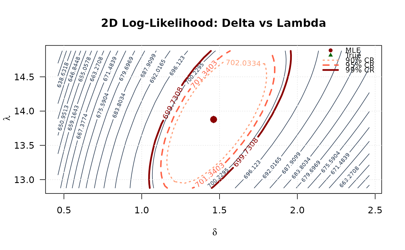
 ## Example 8: 2D Log-Likelihood Surface (Delta vs Lambda)
# Create 2D grid
delta_2d_2 <- seq(mle[4] - xd, mle[4] + xd, length.out = round(n / 30))
lambda_2d <- seq(mle[5] - xd, mle[5] + xd, length.out = round(n / 30))
delta_2d_2 <- delta_2d_2[delta_2d_2 > 0]
lambda_2d <- lambda_2d[lambda_2d > 0]
# Compute log-likelihood surface
ll_surface_dl <- matrix(NA, nrow = length(delta_2d_2), ncol = length(lambda_2d))
for (i in seq_along(delta_2d_2)) {
for (j in seq_along(lambda_2d)) {
ll_surface_dl[i, j] <- -llgkw(c(
mle[1], mle[2], mle[3],
delta_2d_2[i], lambda_2d[j]
), data)
}
}
# Confidence region levels
max_ll_dl <- max(ll_surface_dl, na.rm = TRUE)
levels_90_dl <- max_ll_dl - qchisq(0.90, df = 2) / 2
levels_95_dl <- max_ll_dl - qchisq(0.95, df = 2) / 2
levels_99_dl <- max_ll_dl - qchisq(0.99, df = 2) / 2
# Plot contour
contour(delta_2d_2, lambda_2d, ll_surface_dl,
xlab = expression(delta), ylab = expression(lambda),
main = "2D Log-Likelihood: Delta vs Lambda",
levels = seq(min(ll_surface_dl, na.rm = TRUE), max_ll_dl, length.out = 20),
col = "#2E4057", las = 1, lwd = 1
)
contour(delta_2d_2, lambda_2d, ll_surface_dl,
levels = c(levels_90_dl, levels_95_dl, levels_99_dl),
col = c("#FFA07A", "#FF6347", "#8B0000"),
lwd = c(2, 2.5, 3), lty = c(3, 2, 1),
add = TRUE, labcex = 0.8
)
points(mle[4], mle[5], pch = 19, col = "#8B0000", cex = 1.5)
points(true_params[4], true_params[5], pch = 17, col = "#006400", cex = 1.5)
legend("topright",
legend = c("MLE", "True", "90% CR", "95% CR", "99% CR"),
col = c("#8B0000", "#006400", "#FFA07A", "#FF6347", "#8B0000"),
pch = c(19, 17, NA, NA, NA),
lty = c(NA, NA, 3, 2, 1),
lwd = c(NA, NA, 2, 2.5, 3),
bty = "n", cex = 0.8
)
grid(col = "gray90")
## Example 8: 2D Log-Likelihood Surface (Delta vs Lambda)
# Create 2D grid
delta_2d_2 <- seq(mle[4] - xd, mle[4] + xd, length.out = round(n / 30))
lambda_2d <- seq(mle[5] - xd, mle[5] + xd, length.out = round(n / 30))
delta_2d_2 <- delta_2d_2[delta_2d_2 > 0]
lambda_2d <- lambda_2d[lambda_2d > 0]
# Compute log-likelihood surface
ll_surface_dl <- matrix(NA, nrow = length(delta_2d_2), ncol = length(lambda_2d))
for (i in seq_along(delta_2d_2)) {
for (j in seq_along(lambda_2d)) {
ll_surface_dl[i, j] <- -llgkw(c(
mle[1], mle[2], mle[3],
delta_2d_2[i], lambda_2d[j]
), data)
}
}
# Confidence region levels
max_ll_dl <- max(ll_surface_dl, na.rm = TRUE)
levels_90_dl <- max_ll_dl - qchisq(0.90, df = 2) / 2
levels_95_dl <- max_ll_dl - qchisq(0.95, df = 2) / 2
levels_99_dl <- max_ll_dl - qchisq(0.99, df = 2) / 2
# Plot contour
contour(delta_2d_2, lambda_2d, ll_surface_dl,
xlab = expression(delta), ylab = expression(lambda),
main = "2D Log-Likelihood: Delta vs Lambda",
levels = seq(min(ll_surface_dl, na.rm = TRUE), max_ll_dl, length.out = 20),
col = "#2E4057", las = 1, lwd = 1
)
contour(delta_2d_2, lambda_2d, ll_surface_dl,
levels = c(levels_90_dl, levels_95_dl, levels_99_dl),
col = c("#FFA07A", "#FF6347", "#8B0000"),
lwd = c(2, 2.5, 3), lty = c(3, 2, 1),
add = TRUE, labcex = 0.8
)
points(mle[4], mle[5], pch = 19, col = "#8B0000", cex = 1.5)
points(true_params[4], true_params[5], pch = 17, col = "#006400", cex = 1.5)
legend("topright",
legend = c("MLE", "True", "90% CR", "95% CR", "99% CR"),
col = c("#8B0000", "#006400", "#FFA07A", "#FF6347", "#8B0000"),
pch = c(19, 17, NA, NA, NA),
lty = c(NA, NA, 3, 2, 1),
lwd = c(NA, NA, 2, 2.5, 3),
bty = "n", cex = 0.8
)
grid(col = "gray90")
 # }
# }