Computes the analytic 4x4 Hessian matrix (matrix of second partial derivatives)
of the negative log-likelihood function for the Beta-Kumaraswamy (BKw)
distribution with parameters alpha (\(\alpha\)), beta
(\(\beta\)), gamma (\(\gamma\)), and delta (\(\delta\)).
This distribution is the special case of the Generalized Kumaraswamy (GKw)
distribution where \(\lambda = 1\). The Hessian is useful for estimating
standard errors and in optimization algorithms.
Value
Returns a 4x4 numeric matrix representing the Hessian matrix of the
negative log-likelihood function, \(-\partial^2 \ell / (\partial \theta_i \partial \theta_j)\),
where \(\theta = (\alpha, \beta, \gamma, \delta)\).
Returns a 4x4 matrix populated with NaN if any parameter values are
invalid according to their constraints, or if any value in data is
not in the interval (0, 1).
Details
This function calculates the analytic second partial derivatives of the
negative log-likelihood function based on the BKw log-likelihood
(\(\lambda=1\) case of GKw, see llbkw):
$$
\ell(\theta | \mathbf{x}) = n[\ln(\alpha) + \ln(\beta) - \ln B(\gamma, \delta+1)]
+ \sum_{i=1}^{n} [(\alpha-1)\ln(x_i) + (\beta(\delta+1)-1)\ln(v_i) + (\gamma-1)\ln(w_i)]
$$
where \(\theta = (\alpha, \beta, \gamma, \delta)\), \(B(a,b)\)
is the Beta function (beta), and intermediate terms are:
\(v_i = 1 - x_i^{\alpha}\)
\(w_i = 1 - v_i^{\beta} = 1 - (1-x_i^{\alpha})^{\beta}\)
The Hessian matrix returned contains the elements \(- \frac{\partial^2 \ell(\theta | \mathbf{x})}{\partial \theta_i \partial \theta_j}\) for \(\theta_i, \theta_j \in \{\alpha, \beta, \gamma, \delta\}\).
Key properties of the returned matrix:
Dimensions: 4x4.
Symmetry: The matrix is symmetric.
Ordering: Rows and columns correspond to the parameters in the order \(\alpha, \beta, \gamma, \delta\).
Content: Analytic second derivatives of the negative log-likelihood.
This corresponds to the relevant 4x4 submatrix of the 5x5 GKw Hessian (hsgkw)
evaluated at \(\lambda=1\). The exact analytical formulas are implemented directly.
References
Cordeiro, G. M., & de Castro, M. (2011). A new family of generalized distributions. Journal of Statistical Computation and Simulation,
Kumaraswamy, P. (1980). A generalized probability density function for double-bounded random processes. Journal of Hydrology, 46(1-2), 79-88.
(Note: Specific Hessian formulas might be derived or sourced from additional references).
Examples
# \donttest{
## Example 1: Basic Hessian Evaluation
# Generate sample data
set.seed(2203)
n <- 1000
true_params <- c(alpha = 2.0, beta = 1.5, gamma = 1.5, delta = 0.5)
data <- rbkw(n,
alpha = true_params[1], beta = true_params[2],
gamma = true_params[3], delta = true_params[4]
)
# Evaluate Hessian at true parameters
hess_true <- hsbkw(par = true_params, data = data)
cat("Hessian matrix at true parameters:\n")
#> Hessian matrix at true parameters:
print(hess_true, digits = 4)
#> [,1] [,2] [,3] [,4]
#> [1,] 536.6 -465.2 552.9 -418.2
#> [2,] -465.2 648.7 -447.0 563.2
#> [3,] 552.9 -447.0 539.9 -394.9
#> [4,] -418.2 563.2 -394.9 539.9
# Check symmetry
cat(
"\nSymmetry check (max |H - H^T|):",
max(abs(hess_true - t(hess_true))), "\n"
)
#>
#> Symmetry check (max |H - H^T|): 0
## Example 2: Hessian Properties at MLE
# Fit model
fit <- optim(
par = c(1.8, 1.2, 1.1, 0.3),
fn = llbkw,
gr = grbkw,
data = data,
method = "Nelder-Mead",
hessian = TRUE
)
mle <- fit$par
names(mle) <- c("alpha", "beta", "gamma", "delta")
# Hessian at MLE
hessian_at_mle <- hsbkw(par = mle, data = data)
cat("\nHessian at MLE:\n")
#>
#> Hessian at MLE:
print(hessian_at_mle, digits = 4)
#> [,1] [,2] [,3] [,4]
#> [1,] 337.7 -205.4 516.6 -433.8
#> [2,] -205.4 203.8 -273.5 433.1
#> [3,] 516.6 -273.5 816.6 -576.4
#> [4,] -433.8 433.1 -576.4 920.9
# Compare with optim's numerical Hessian
cat("\nComparison with optim Hessian:\n")
#>
#> Comparison with optim Hessian:
cat(
"Max absolute difference:",
max(abs(hessian_at_mle - fit$hessian)), "\n"
)
#> Max absolute difference: 0.0007850156
# Eigenvalue analysis
eigenvals <- eigen(hessian_at_mle, only.values = TRUE)$values
cat("\nEigenvalues:\n")
#>
#> Eigenvalues:
print(eigenvals)
#> [1] 1932.6299085 345.0426785 1.2086682 0.1217554
cat("\nPositive definite:", all(eigenvals > 0), "\n")
#>
#> Positive definite: TRUE
cat("Condition number:", max(eigenvals) / min(eigenvals), "\n")
#> Condition number: 15873.05
## Example 3: Standard Errors and Confidence Intervals
# Observed information matrix
obs_info <- hessian_at_mle
# Variance-covariance matrix
vcov_matrix <- solve(obs_info)
cat("\nVariance-Covariance Matrix:\n")
#>
#> Variance-Covariance Matrix:
print(vcov_matrix, digits = 6)
#> [,1] [,2] [,3] [,4]
#> [1,] 0.63827083 0.1882004 -0.3421762 -0.00197877
#> [2,] 0.18820037 6.7563286 -0.0657884 -3.13009829
#> [3,] -0.34217618 -0.0657884 0.1858182 -0.01396138
#> [4,] -0.00197877 -3.1300983 -0.0139614 1.46353994
# Standard errors
se <- sqrt(diag(vcov_matrix))
names(se) <- c("alpha", "beta", "gamma", "delta")
# Correlation matrix
corr_matrix <- cov2cor(vcov_matrix)
cat("\nCorrelation Matrix:\n")
#>
#> Correlation Matrix:
print(corr_matrix, digits = 4)
#> [,1] [,2] [,3] [,4]
#> [1,] 1.000000 0.09063 -0.99358 -0.002047
#> [2,] 0.090628 1.00000 -0.05872 -0.995406
#> [3,] -0.993581 -0.05872 1.00000 -0.026772
#> [4,] -0.002047 -0.99541 -0.02677 1.000000
# Confidence intervals
z_crit <- qnorm(0.975)
results <- data.frame(
Parameter = c("alpha", "beta", "gamma", "delta"),
True = true_params,
MLE = mle,
SE = se,
CI_Lower = mle - z_crit * se,
CI_Upper = mle + z_crit * se
)
print(results, digits = 4)
#> Parameter True MLE SE CI_Lower CI_Upper
#> alpha alpha 2.0 2.57049 0.7989 1.0046 4.136
#> beta beta 1.5 2.33192 2.5993 -2.7626 7.426
#> gamma gamma 1.5 1.12226 0.4311 0.2774 1.967
#> delta delta 0.5 0.06702 1.2098 -2.3041 2.438
## Example 4: Determinant and Trace Analysis
# Compute at different points
test_params <- rbind(
c(1.5, 1.0, 1.0, 0.3),
c(2.0, 1.5, 1.5, 0.5),
mle,
c(2.5, 2.0, 2.0, 0.7)
)
hess_properties <- data.frame(
Alpha = numeric(),
Beta = numeric(),
Gamma = numeric(),
Delta = numeric(),
Determinant = numeric(),
Trace = numeric(),
Min_Eigenval = numeric(),
Max_Eigenval = numeric(),
Cond_Number = numeric(),
stringsAsFactors = FALSE
)
for (i in 1:nrow(test_params)) {
H <- hsbkw(par = test_params[i, ], data = data)
eigs <- eigen(H, only.values = TRUE)$values
hess_properties <- rbind(hess_properties, data.frame(
Alpha = test_params[i, 1],
Beta = test_params[i, 2],
Gamma = test_params[i, 3],
Delta = test_params[i, 4],
Determinant = det(H),
Trace = sum(diag(H)),
Min_Eigenval = min(eigs),
Max_Eigenval = max(eigs),
Cond_Number = max(eigs) / min(eigs)
))
}
cat("\nHessian Properties at Different Points:\n")
#>
#> Hessian Properties at Different Points:
print(hess_properties, digits = 4, row.names = FALSE)
#> Alpha Beta Gamma Delta Determinant Trace Min_Eigenval Max_Eigenval
#> 1.50 1.000 1.000 0.30000 -6.191e+10 3261 -134.1926 2027
#> 2.00 1.500 1.500 0.50000 -2.362e+08 2265 -15.8487 1990
#> 2.57 2.332 1.122 0.06702 9.813e+04 2279 0.1218 1933
#> 2.50 2.000 2.000 0.70000 -1.510e+09 1805 -118.6118 1662
#> Cond_Number
#> -15.10
#> -125.59
#> 15873.05
#> -14.01
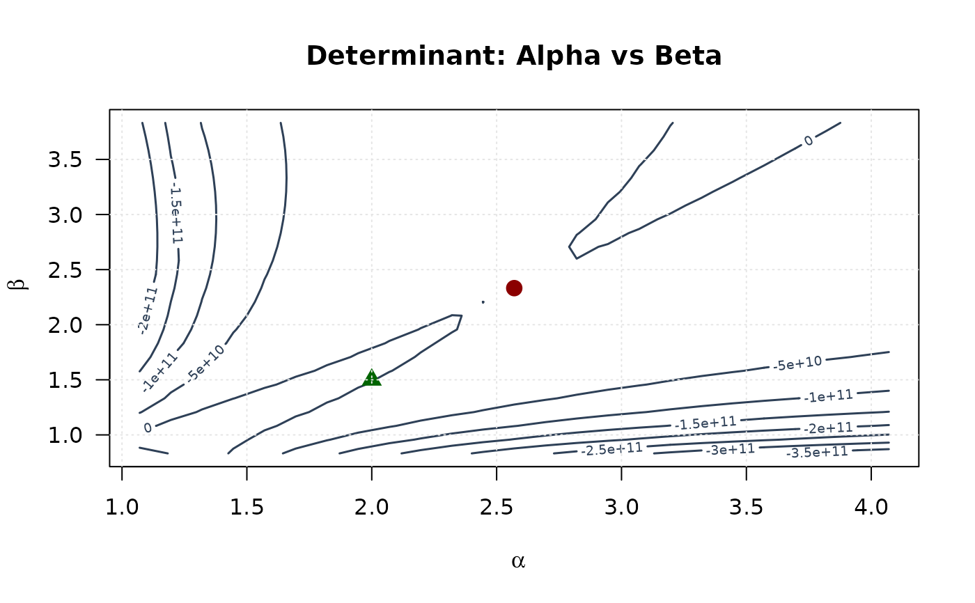
## Example 5: Curvature Visualization (Selected pairs)
# Create grids around MLE with wider range (±1.5)
alpha_grid <- seq(mle[1] - 1.5, mle[1] + 1.5, length.out = 25)
beta_grid <- seq(mle[2] - 1.5, mle[2] + 1.5, length.out = 25)
gamma_grid <- seq(mle[3] - 1.5, mle[3] + 1.5, length.out = 25)
delta_grid <- seq(mle[4] - 1.5, mle[4] + 1.5, length.out = 25)
alpha_grid <- alpha_grid[alpha_grid > 0]
beta_grid <- beta_grid[beta_grid > 0]
gamma_grid <- gamma_grid[gamma_grid > 0]
delta_grid <- delta_grid[delta_grid > 0]
# Compute curvature measures for selected pairs
determinant_surface_ab <- matrix(NA, nrow = length(alpha_grid), ncol = length(beta_grid))
trace_surface_ab <- matrix(NA, nrow = length(alpha_grid), ncol = length(beta_grid))
determinant_surface_ag <- matrix(NA, nrow = length(alpha_grid), ncol = length(gamma_grid))
trace_surface_ag <- matrix(NA, nrow = length(alpha_grid), ncol = length(gamma_grid))
determinant_surface_bd <- matrix(NA, nrow = length(beta_grid), ncol = length(delta_grid))
trace_surface_bd <- matrix(NA, nrow = length(beta_grid), ncol = length(delta_grid))
# Alpha vs Beta
for (i in seq_along(alpha_grid)) {
for (j in seq_along(beta_grid)) {
H <- hsbkw(c(alpha_grid[i], beta_grid[j], mle[3], mle[4]), data)
determinant_surface_ab[i, j] <- det(H)
trace_surface_ab[i, j] <- sum(diag(H))
}
}
# Alpha vs Gamma
for (i in seq_along(alpha_grid)) {
for (j in seq_along(gamma_grid)) {
H <- hsbkw(c(alpha_grid[i], mle[2], gamma_grid[j], mle[4]), data)
determinant_surface_ag[i, j] <- det(H)
trace_surface_ag[i, j] <- sum(diag(H))
}
}
# Beta vs Delta
for (i in seq_along(beta_grid)) {
for (j in seq_along(delta_grid)) {
H <- hsbkw(c(mle[1], beta_grid[i], mle[3], delta_grid[j]), data)
determinant_surface_bd[i, j] <- det(H)
trace_surface_bd[i, j] <- sum(diag(H))
}
}
# Plot selected curvature surfaces
# Determinant plots
contour(alpha_grid, beta_grid, determinant_surface_ab,
xlab = expression(alpha), ylab = expression(beta),
main = "Determinant: Alpha vs Beta", las = 1,
col = "#2E4057", lwd = 1.5, nlevels = 15
)
points(mle[1], mle[2], pch = 19, col = "#8B0000", cex = 1.5)
points(true_params[1], true_params[2], pch = 17, col = "#006400", cex = 1.5)
grid(col = "gray90")
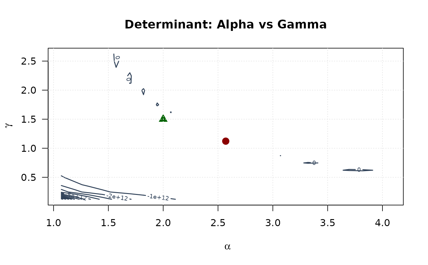
 contour(alpha_grid, gamma_grid, determinant_surface_ag,
xlab = expression(alpha), ylab = expression(gamma),
main = "Determinant: Alpha vs Gamma", las = 1,
col = "#2E4057", lwd = 1.5, nlevels = 15
)
points(mle[1], mle[3], pch = 19, col = "#8B0000", cex = 1.5)
points(true_params[1], true_params[3], pch = 17, col = "#006400", cex = 1.5)
grid(col = "gray90")
contour(alpha_grid, gamma_grid, determinant_surface_ag,
xlab = expression(alpha), ylab = expression(gamma),
main = "Determinant: Alpha vs Gamma", las = 1,
col = "#2E4057", lwd = 1.5, nlevels = 15
)
points(mle[1], mle[3], pch = 19, col = "#8B0000", cex = 1.5)
points(true_params[1], true_params[3], pch = 17, col = "#006400", cex = 1.5)
grid(col = "gray90")
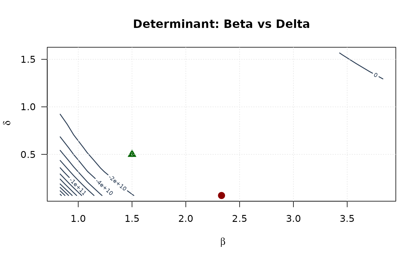
 contour(beta_grid, delta_grid, determinant_surface_bd,
xlab = expression(beta), ylab = expression(delta),
main = "Determinant: Beta vs Delta", las = 1,
col = "#2E4057", lwd = 1.5, nlevels = 15
)
points(mle[2], mle[4], pch = 19, col = "#8B0000", cex = 1.5)
points(true_params[2], true_params[4], pch = 17, col = "#006400", cex = 1.5)
grid(col = "gray90")
contour(beta_grid, delta_grid, determinant_surface_bd,
xlab = expression(beta), ylab = expression(delta),
main = "Determinant: Beta vs Delta", las = 1,
col = "#2E4057", lwd = 1.5, nlevels = 15
)
points(mle[2], mle[4], pch = 19, col = "#8B0000", cex = 1.5)
points(true_params[2], true_params[4], pch = 17, col = "#006400", cex = 1.5)
grid(col = "gray90")
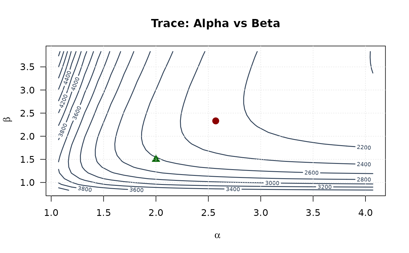
 # Trace plots
contour(alpha_grid, beta_grid, trace_surface_ab,
xlab = expression(alpha), ylab = expression(beta),
main = "Trace: Alpha vs Beta", las = 1,
col = "#2E4057", lwd = 1.5, nlevels = 15
)
points(mle[1], mle[2], pch = 19, col = "#8B0000", cex = 1.5)
points(true_params[1], true_params[2], pch = 17, col = "#006400", cex = 1.5)
grid(col = "gray90")
# Trace plots
contour(alpha_grid, beta_grid, trace_surface_ab,
xlab = expression(alpha), ylab = expression(beta),
main = "Trace: Alpha vs Beta", las = 1,
col = "#2E4057", lwd = 1.5, nlevels = 15
)
points(mle[1], mle[2], pch = 19, col = "#8B0000", cex = 1.5)
points(true_params[1], true_params[2], pch = 17, col = "#006400", cex = 1.5)
grid(col = "gray90")
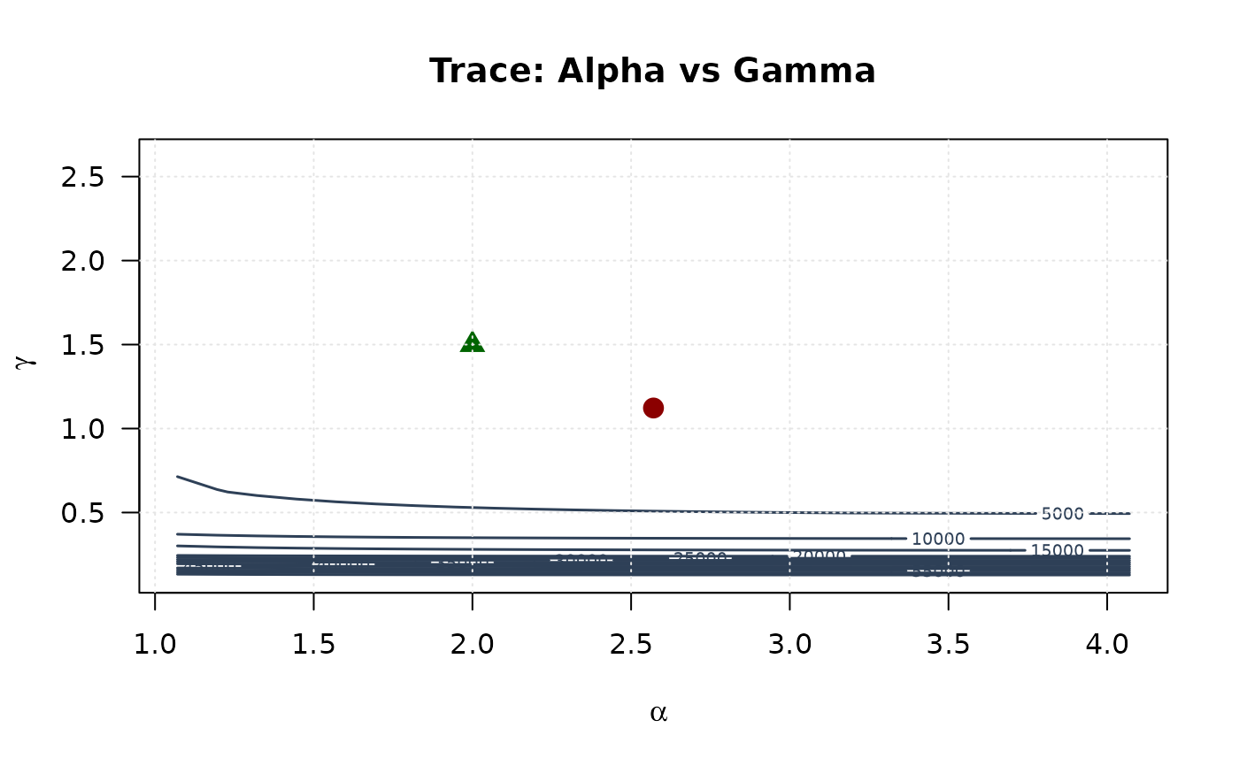
 contour(alpha_grid, gamma_grid, trace_surface_ag,
xlab = expression(alpha), ylab = expression(gamma),
main = "Trace: Alpha vs Gamma", las = 1,
col = "#2E4057", lwd = 1.5, nlevels = 15
)
points(mle[1], mle[3], pch = 19, col = "#8B0000", cex = 1.5)
points(true_params[1], true_params[3], pch = 17, col = "#006400", cex = 1.5)
grid(col = "gray90")
contour(alpha_grid, gamma_grid, trace_surface_ag,
xlab = expression(alpha), ylab = expression(gamma),
main = "Trace: Alpha vs Gamma", las = 1,
col = "#2E4057", lwd = 1.5, nlevels = 15
)
points(mle[1], mle[3], pch = 19, col = "#8B0000", cex = 1.5)
points(true_params[1], true_params[3], pch = 17, col = "#006400", cex = 1.5)
grid(col = "gray90")
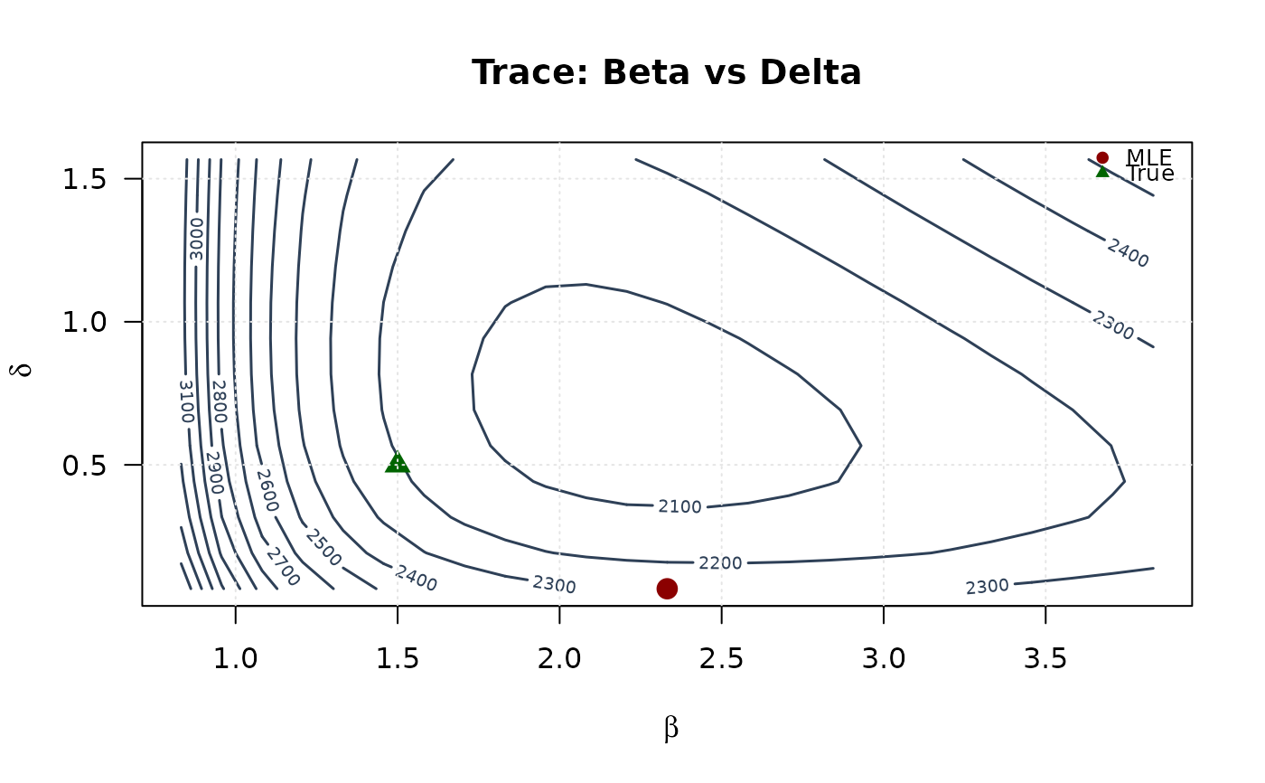
 contour(beta_grid, delta_grid, trace_surface_bd,
xlab = expression(beta), ylab = expression(delta),
main = "Trace: Beta vs Delta", las = 1,
col = "#2E4057", lwd = 1.5, nlevels = 15
)
points(mle[2], mle[4], pch = 19, col = "#8B0000", cex = 1.5)
points(true_params[2], true_params[4], pch = 17, col = "#006400", cex = 1.5)
grid(col = "gray90")
legend("topright",
legend = c("MLE", "True"),
col = c("#8B0000", "#006400"),
pch = c(19, 17),
bty = "n", cex = 0.8
)
contour(beta_grid, delta_grid, trace_surface_bd,
xlab = expression(beta), ylab = expression(delta),
main = "Trace: Beta vs Delta", las = 1,
col = "#2E4057", lwd = 1.5, nlevels = 15
)
points(mle[2], mle[4], pch = 19, col = "#8B0000", cex = 1.5)
points(true_params[2], true_params[4], pch = 17, col = "#006400", cex = 1.5)
grid(col = "gray90")
legend("topright",
legend = c("MLE", "True"),
col = c("#8B0000", "#006400"),
pch = c(19, 17),
bty = "n", cex = 0.8
)
 ## Example 6: Confidence Ellipses (Selected pairs)
# Extract selected 2x2 submatrices
vcov_ab <- vcov_matrix[1:2, 1:2]
vcov_ag <- vcov_matrix[c(1, 3), c(1, 3)]
vcov_bd <- vcov_matrix[c(2, 4), c(2, 4)]
# Create confidence ellipses
theta <- seq(0, 2 * pi, length.out = 100)
chi2_val <- qchisq(0.95, df = 2)
# Alpha vs Beta ellipse
eig_decomp_ab <- eigen(vcov_ab)
ellipse_ab <- matrix(NA, nrow = 100, ncol = 2)
for (i in 1:100) {
v <- c(cos(theta[i]), sin(theta[i]))
ellipse_ab[i, ] <- mle[1:2] + sqrt(chi2_val) *
(eig_decomp_ab$vectors %*% diag(sqrt(eig_decomp_ab$values)) %*% v)
}
# Alpha vs Gamma ellipse
eig_decomp_ag <- eigen(vcov_ag)
ellipse_ag <- matrix(NA, nrow = 100, ncol = 2)
for (i in 1:100) {
v <- c(cos(theta[i]), sin(theta[i]))
ellipse_ag[i, ] <- mle[c(1, 3)] + sqrt(chi2_val) *
(eig_decomp_ag$vectors %*% diag(sqrt(eig_decomp_ag$values)) %*% v)
}
# Beta vs Delta ellipse
eig_decomp_bd <- eigen(vcov_bd)
ellipse_bd <- matrix(NA, nrow = 100, ncol = 2)
for (i in 1:100) {
v <- c(cos(theta[i]), sin(theta[i]))
ellipse_bd[i, ] <- mle[c(2, 4)] + sqrt(chi2_val) *
(eig_decomp_bd$vectors %*% diag(sqrt(eig_decomp_bd$values)) %*% v)
}
# Marginal confidence intervals
se_ab <- sqrt(diag(vcov_ab))
ci_alpha_ab <- mle[1] + c(-1, 1) * 1.96 * se_ab[1]
ci_beta_ab <- mle[2] + c(-1, 1) * 1.96 * se_ab[2]
se_ag <- sqrt(diag(vcov_ag))
ci_alpha_ag <- mle[1] + c(-1, 1) * 1.96 * se_ag[1]
ci_gamma_ag <- mle[3] + c(-1, 1) * 1.96 * se_ag[2]
se_bd <- sqrt(diag(vcov_bd))
ci_beta_bd <- mle[2] + c(-1, 1) * 1.96 * se_bd[1]
ci_delta_bd <- mle[4] + c(-1, 1) * 1.96 * se_bd[2]
# Plot selected ellipses side by side
# Alpha vs Beta
plot(ellipse_ab[, 1], ellipse_ab[, 2],
type = "l", lwd = 2, col = "#2E4057",
xlab = expression(alpha), ylab = expression(beta),
main = "Alpha vs Beta", las = 1, xlim = range(ellipse_ab[, 1], ci_alpha_ab),
ylim = range(ellipse_ab[, 2], ci_beta_ab)
)
abline(v = ci_alpha_ab, col = "#808080", lty = 3, lwd = 1.5)
abline(h = ci_beta_ab, col = "#808080", lty = 3, lwd = 1.5)
points(mle[1], mle[2], pch = 19, col = "#8B0000", cex = 1.5)
points(true_params[1], true_params[2], pch = 17, col = "#006400", cex = 1.5)
grid(col = "gray90")
## Example 6: Confidence Ellipses (Selected pairs)
# Extract selected 2x2 submatrices
vcov_ab <- vcov_matrix[1:2, 1:2]
vcov_ag <- vcov_matrix[c(1, 3), c(1, 3)]
vcov_bd <- vcov_matrix[c(2, 4), c(2, 4)]
# Create confidence ellipses
theta <- seq(0, 2 * pi, length.out = 100)
chi2_val <- qchisq(0.95, df = 2)
# Alpha vs Beta ellipse
eig_decomp_ab <- eigen(vcov_ab)
ellipse_ab <- matrix(NA, nrow = 100, ncol = 2)
for (i in 1:100) {
v <- c(cos(theta[i]), sin(theta[i]))
ellipse_ab[i, ] <- mle[1:2] + sqrt(chi2_val) *
(eig_decomp_ab$vectors %*% diag(sqrt(eig_decomp_ab$values)) %*% v)
}
# Alpha vs Gamma ellipse
eig_decomp_ag <- eigen(vcov_ag)
ellipse_ag <- matrix(NA, nrow = 100, ncol = 2)
for (i in 1:100) {
v <- c(cos(theta[i]), sin(theta[i]))
ellipse_ag[i, ] <- mle[c(1, 3)] + sqrt(chi2_val) *
(eig_decomp_ag$vectors %*% diag(sqrt(eig_decomp_ag$values)) %*% v)
}
# Beta vs Delta ellipse
eig_decomp_bd <- eigen(vcov_bd)
ellipse_bd <- matrix(NA, nrow = 100, ncol = 2)
for (i in 1:100) {
v <- c(cos(theta[i]), sin(theta[i]))
ellipse_bd[i, ] <- mle[c(2, 4)] + sqrt(chi2_val) *
(eig_decomp_bd$vectors %*% diag(sqrt(eig_decomp_bd$values)) %*% v)
}
# Marginal confidence intervals
se_ab <- sqrt(diag(vcov_ab))
ci_alpha_ab <- mle[1] + c(-1, 1) * 1.96 * se_ab[1]
ci_beta_ab <- mle[2] + c(-1, 1) * 1.96 * se_ab[2]
se_ag <- sqrt(diag(vcov_ag))
ci_alpha_ag <- mle[1] + c(-1, 1) * 1.96 * se_ag[1]
ci_gamma_ag <- mle[3] + c(-1, 1) * 1.96 * se_ag[2]
se_bd <- sqrt(diag(vcov_bd))
ci_beta_bd <- mle[2] + c(-1, 1) * 1.96 * se_bd[1]
ci_delta_bd <- mle[4] + c(-1, 1) * 1.96 * se_bd[2]
# Plot selected ellipses side by side
# Alpha vs Beta
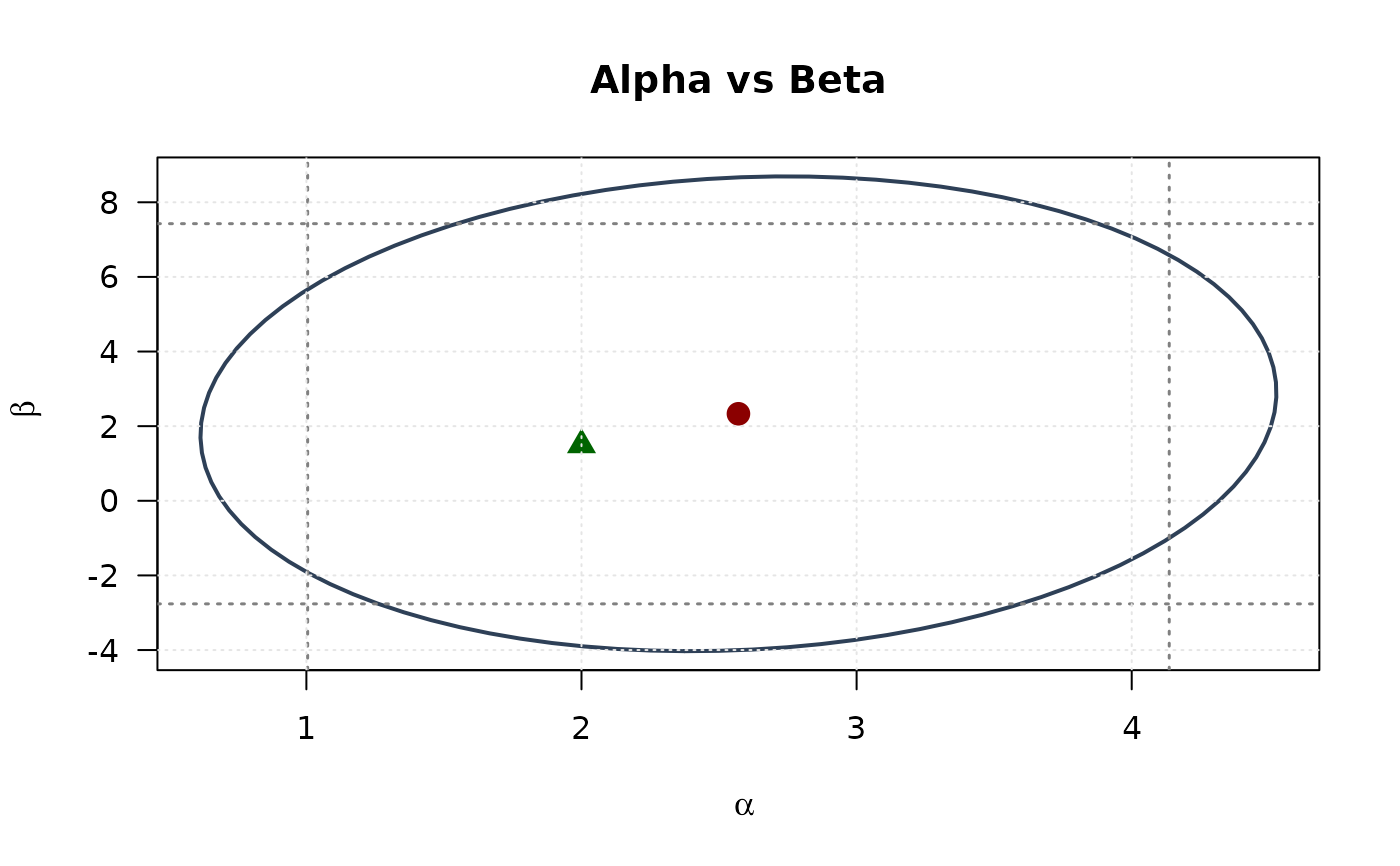
plot(ellipse_ab[, 1], ellipse_ab[, 2],
type = "l", lwd = 2, col = "#2E4057",
xlab = expression(alpha), ylab = expression(beta),
main = "Alpha vs Beta", las = 1, xlim = range(ellipse_ab[, 1], ci_alpha_ab),
ylim = range(ellipse_ab[, 2], ci_beta_ab)
)
abline(v = ci_alpha_ab, col = "#808080", lty = 3, lwd = 1.5)
abline(h = ci_beta_ab, col = "#808080", lty = 3, lwd = 1.5)
points(mle[1], mle[2], pch = 19, col = "#8B0000", cex = 1.5)
points(true_params[1], true_params[2], pch = 17, col = "#006400", cex = 1.5)
grid(col = "gray90")
 # Alpha vs Gamma
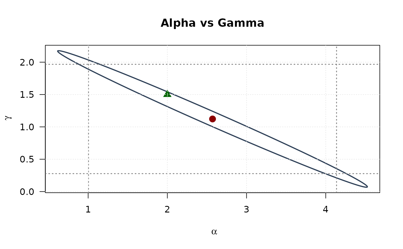
plot(ellipse_ag[, 1], ellipse_ag[, 2],
type = "l", lwd = 2, col = "#2E4057",
xlab = expression(alpha), ylab = expression(gamma),
main = "Alpha vs Gamma", las = 1, xlim = range(ellipse_ag[, 1], ci_alpha_ag),
ylim = range(ellipse_ag[, 2], ci_gamma_ag)
)
abline(v = ci_alpha_ag, col = "#808080", lty = 3, lwd = 1.5)
abline(h = ci_gamma_ag, col = "#808080", lty = 3, lwd = 1.5)
points(mle[1], mle[3], pch = 19, col = "#8B0000", cex = 1.5)
points(true_params[1], true_params[3], pch = 17, col = "#006400", cex = 1.5)
grid(col = "gray90")
# Alpha vs Gamma
plot(ellipse_ag[, 1], ellipse_ag[, 2],
type = "l", lwd = 2, col = "#2E4057",
xlab = expression(alpha), ylab = expression(gamma),
main = "Alpha vs Gamma", las = 1, xlim = range(ellipse_ag[, 1], ci_alpha_ag),
ylim = range(ellipse_ag[, 2], ci_gamma_ag)
)
abline(v = ci_alpha_ag, col = "#808080", lty = 3, lwd = 1.5)
abline(h = ci_gamma_ag, col = "#808080", lty = 3, lwd = 1.5)
points(mle[1], mle[3], pch = 19, col = "#8B0000", cex = 1.5)
points(true_params[1], true_params[3], pch = 17, col = "#006400", cex = 1.5)
grid(col = "gray90")
 # Beta vs Delta
plot(ellipse_bd[, 1], ellipse_bd[, 2],
type = "l", lwd = 2, col = "#2E4057",
xlab = expression(beta), ylab = expression(delta),
main = "Beta vs Delta", las = 1, xlim = range(ellipse_bd[, 1], ci_beta_bd),
ylim = range(ellipse_bd[, 2], ci_delta_bd)
)
abline(v = ci_beta_bd, col = "#808080", lty = 3, lwd = 1.5)
abline(h = ci_delta_bd, col = "#808080", lty = 3, lwd = 1.5)
points(mle[2], mle[4], pch = 19, col = "#8B0000", cex = 1.5)
points(true_params[2], true_params[4], pch = 17, col = "#006400", cex = 1.5)
grid(col = "gray90")
legend("topright",
legend = c("MLE", "True", "95% CR", "Marginal 95% CI"),
col = c("#8B0000", "#006400", "#2E4057", "#808080"),
pch = c(19, 17, NA, NA),
lty = c(NA, NA, 1, 3),
lwd = c(NA, NA, 2, 1.5),
bty = "n", cex = 0.8
)
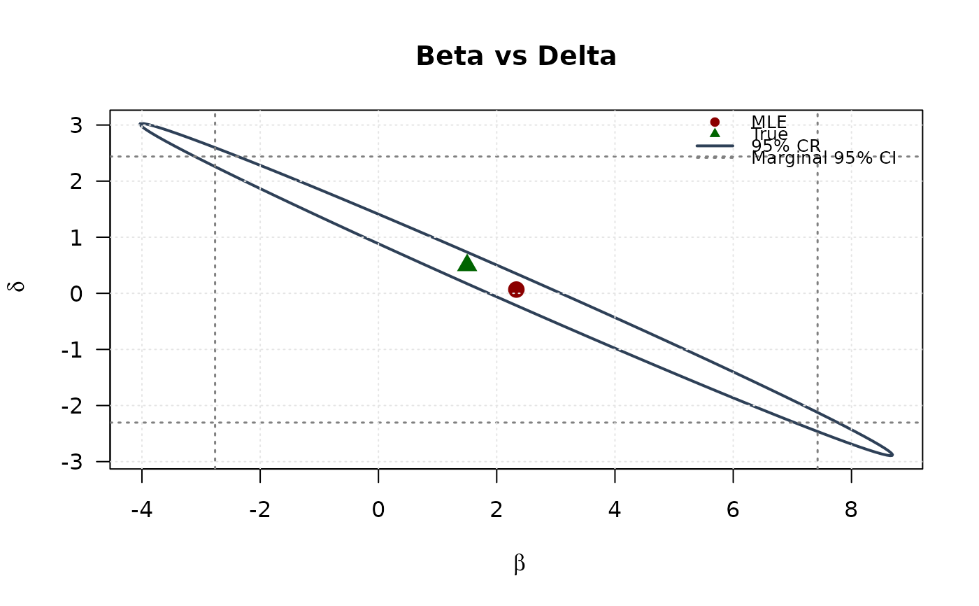
# Beta vs Delta
plot(ellipse_bd[, 1], ellipse_bd[, 2],
type = "l", lwd = 2, col = "#2E4057",
xlab = expression(beta), ylab = expression(delta),
main = "Beta vs Delta", las = 1, xlim = range(ellipse_bd[, 1], ci_beta_bd),
ylim = range(ellipse_bd[, 2], ci_delta_bd)
)
abline(v = ci_beta_bd, col = "#808080", lty = 3, lwd = 1.5)
abline(h = ci_delta_bd, col = "#808080", lty = 3, lwd = 1.5)
points(mle[2], mle[4], pch = 19, col = "#8B0000", cex = 1.5)
points(true_params[2], true_params[4], pch = 17, col = "#006400", cex = 1.5)
grid(col = "gray90")
legend("topright",
legend = c("MLE", "True", "95% CR", "Marginal 95% CI"),
col = c("#8B0000", "#006400", "#2E4057", "#808080"),
pch = c(19, 17, NA, NA),
lty = c(NA, NA, 1, 3),
lwd = c(NA, NA, 2, 1.5),
bty = "n", cex = 0.8
)
 # }
# }