Gradient of the Negative Log-Likelihood for the BKw Distribution

Computes the gradient vector (vector of first partial derivatives) of the negative log-likelihood function for the Beta-Kumaraswamy (BKw) distribution with parameters alpha ($\alpha$), beta ($\beta$), gamma ($\gamma$), and delta ($\delta$). This distribution is the special case of the Generalized Kumaraswamy (GKw) distribution where $\lambda = 1$. The gradient is typically used in optimization algorithms for maximum likelihood estimation.

Usage

grbkw(par, data)

Arguments

par: A numeric vector of length 4 containing the distribution parameters in the order: alpha ($\alpha > 0$), beta ($\beta > 0$), gamma ($\gamma > 0$), delta ($\delta \ge 0$).
data: A numeric vector of observations. All values must be strictly between 0 and 1 (exclusive).

Value

Returns a numeric vector of length 4 containing the partial derivatives of the negative log-likelihood function $-\ell(\theta | \mathbf{x})$ with respect to each parameter: $(-\partial \ell/\partial \alpha, -\partial \ell/\partial \beta, -\partial \ell/\partial \gamma, -\partial \ell/\partial \delta)$. Returns a vector of NaN if any parameter values are invalid according to their constraints, or if any value in data is not in the interval (0, 1).

Details

The components of the gradient vector of the negative log-likelihood ($-\nabla \ell(\theta | \mathbf{x})$) for the BKw ($\lambda=1$) model are:

$$ -\frac{\partial \ell}{\partial \alpha} = -\frac{n}{\alpha} - \sum_{i=1}^{n}\ln(x_i) + \sum_{i=1}^{n}\left[x_i^{\alpha} \ln(x_i) \left(\frac{\beta(\delta+1)-1}{v_i} - \frac{(\gamma-1) \beta v_i^{\beta-1}}{w_i}\right)\right] $$ $$ -\frac{\partial \ell}{\partial \beta} = -\frac{n}{\beta} - (\delta+1)\sum_{i=1}^{n}\ln(v_i) + \sum_{i=1}^{n}\left[\frac{(\gamma-1) v_i^{\beta} \ln(v_i)}{w_i}\right] $$ $$ -\frac{\partial \ell}{\partial \gamma} = n[\psi(\gamma) - \psi(\gamma+\delta+1)] - \sum_{i=1}^{n}\ln(w_i) $$ $$ -\frac{\partial \ell}{\partial \delta} = n[\psi(\delta+1) - \psi(\gamma+\delta+1)] - \beta\sum_{i=1}^{n}\ln(v_i) $$

where:

$v_i = 1 - x_i^{\alpha}$
$w_i = 1 - v_i^{\beta} = 1 - (1-x_i^{\alpha})^{\beta}$
$\psi(\cdot)$ is the digamma function (digamma).

These formulas represent the derivatives of $-\ell(\theta)$, consistent with minimizing the negative log-likelihood. They correspond to the general GKw gradient (grgkw) components for $\alpha, \beta, \gamma, \delta$ evaluated at $\lambda=1$. Note that the component for $\lambda$ is omitted. Numerical stability is maintained through careful implementation.

References

Cordeiro, G. M., & de Castro, M. (2011). A new family of generalized distributions. Journal of Statistical Computation and Simulation,

Kumaraswamy, P. (1980). A generalized probability density function for double-bounded random processes. Journal of Hydrology, 46(1-2), 79-88.

(Note: Specific gradient formulas might be derived or sourced from additional references).

Author

Lopes, J. E.

Examples

# \donttest{
## Example 1: Basic Gradient Evaluation
# Generate sample data
set.seed(2203)
n <- 1000
true_params <- c(alpha = 2.0, beta = 1.5, gamma = 1.5, delta = 0.5)
data <- rbkw(n, alpha = true_params[1], beta = true_params[2],
             gamma = true_params[3], delta = true_params[4])

# Evaluate gradient at true parameters
grad_true <- grbkw(par = true_params, data = data)
cat("Gradient at true parameters:\n")
#> Gradient at true parameters:
print(grad_true)
#> [1]  31.18587 -45.45918  29.19980 -41.56769
cat("Norm:", sqrt(sum(grad_true^2)), "\n")
#> Norm: 74.96397 

# Evaluate at different parameter values
test_params <- rbind(
  c(1.5, 1.0, 1.0, 0.3),
  c(2.0, 1.5, 1.5, 0.5),
  c(2.5, 2.0, 2.0, 0.7)
)

grad_norms <- apply(test_params, 1, function(p) {
  g <- grbkw(p, data)
  sqrt(sum(g^2))
})

results <- data.frame(
  Alpha = test_params[, 1],
  Beta = test_params[, 2],
  Gamma = test_params[, 3],
  Delta = test_params[, 4],
  Grad_Norm = grad_norms
)
print(results, digits = 4)
#>   Alpha Beta Gamma Delta Grad_Norm
#> 1   1.5  1.0   1.0   0.3    337.55
#> 2   2.0  1.5   1.5   0.5     74.96
#> 3   2.5  2.0   2.0   0.7    380.04


## Example 2: Gradient in Optimization

# Optimization with analytical gradient
fit_with_grad <- optim(
  par = c(1.8, 1.2, 1.1, 0.3),
  fn = llbkw,
  gr = grbkw,
  data = data,
  method = "Nelder-Mead",
  hessian = TRUE,
  control = list(trace = 0)
)

# Optimization without gradient
fit_no_grad <- optim(
  par = c(1.8, 1.2, 1.1, 0.3),
  fn = llbkw,
  data = data,
  method = "Nelder-Mead",
  hessian = TRUE,
  control = list(trace = 0)
)

comparison <- data.frame(
  Method = c("With Gradient", "Without Gradient"),
  Alpha = c(fit_with_grad$par[1], fit_no_grad$par[1]),
  Beta = c(fit_with_grad$par[2], fit_no_grad$par[2]),
  Gamma = c(fit_with_grad$par[3], fit_no_grad$par[3]),
  Delta = c(fit_with_grad$par[4], fit_no_grad$par[4]),
  NegLogLik = c(fit_with_grad$value, fit_no_grad$value),
  Iterations = c(fit_with_grad$counts[1], fit_no_grad$counts[1])
)
print(comparison, digits = 4, row.names = FALSE)
#>            Method Alpha  Beta Gamma   Delta NegLogLik Iterations
#>     With Gradient  2.57 2.332 1.122 0.06702    -270.2        501
#>  Without Gradient  2.57 2.332 1.122 0.06702    -270.2        501


## Example 3: Verifying Gradient at MLE

mle <- fit_with_grad$par
names(mle) <- c("alpha", "beta", "gamma", "delta")

# At MLE, gradient should be approximately zero
gradient_at_mle <- grbkw(par = mle, data = data)
cat("\nGradient at MLE:\n")
#> 
#> Gradient at MLE:
print(gradient_at_mle)
#> [1]  0.5000681 -0.1496257  0.6667976 -0.2655980
cat("Max absolute component:", max(abs(gradient_at_mle)), "\n")
#> Max absolute component: 0.6667976 
cat("Gradient norm:", sqrt(sum(gradient_at_mle^2)), "\n")
#> Gradient norm: 0.8874781 


## Example 4: Numerical vs Analytical Gradient

# Manual finite difference gradient
numerical_gradient <- function(f, x, data, h = 1e-7) {
  grad <- numeric(length(x))
  for (i in seq_along(x)) {
    x_plus <- x_minus <- x
    x_plus[i] <- x[i] + h
    x_minus[i] <- x[i] - h
    grad[i] <- (f(x_plus, data) - f(x_minus, data)) / (2 * h)
  }
  return(grad)
}

# Compare at MLE
grad_analytical <- grbkw(par = mle, data = data)
grad_numerical <- numerical_gradient(llbkw, mle, data)

comparison_grad <- data.frame(
  Parameter = c("alpha", "beta", "gamma", "delta"),
  Analytical = grad_analytical,
  Numerical = grad_numerical,
  Abs_Diff = abs(grad_analytical - grad_numerical),
  Rel_Error = abs(grad_analytical - grad_numerical) /
              (abs(grad_analytical) + 1e-10)
)
print(comparison_grad, digits = 8)
#>   Parameter  Analytical   Numerical      Abs_Diff     Rel_Error
#> 1     alpha  0.50006808  0.50006093 7.1441844e-06 1.4286424e-05
#> 2      beta -0.14962570 -0.14962154 4.1532289e-06 2.7757458e-05
#> 3     gamma  0.66679761  0.66679576 1.8569186e-06 2.7848309e-06
#> 4     delta -0.26559804 -0.26560144 3.4024424e-06 1.2810495e-05


## Example 5: Score Test Statistic

# Score test for H0: theta = theta0
theta0 <- c(1.8, 1.3, 1.2, 0.4)
score_theta0 <- -grbkw(par = theta0, data = data)

# Fisher information at theta0
fisher_info <- hsbkw(par = theta0, data = data)

# Score test statistic
score_stat <- t(score_theta0) %*% solve(fisher_info) %*% score_theta0
p_value <- pchisq(score_stat, df = 4, lower.tail = FALSE)

cat("\nScore Test:\n")
#> 
#> Score Test:
cat("H0: alpha=1.8, beta=1.3, gamma=1.2, delta=0.4\n")
#> H0: alpha=1.8, beta=1.3, gamma=1.2, delta=0.4
cat("Test statistic:", score_stat, "\n")
#> Test statistic: 61.34372 
cat("P-value:", format.pval(p_value, digits = 4), "\n")
#> P-value: 1.514e-12 


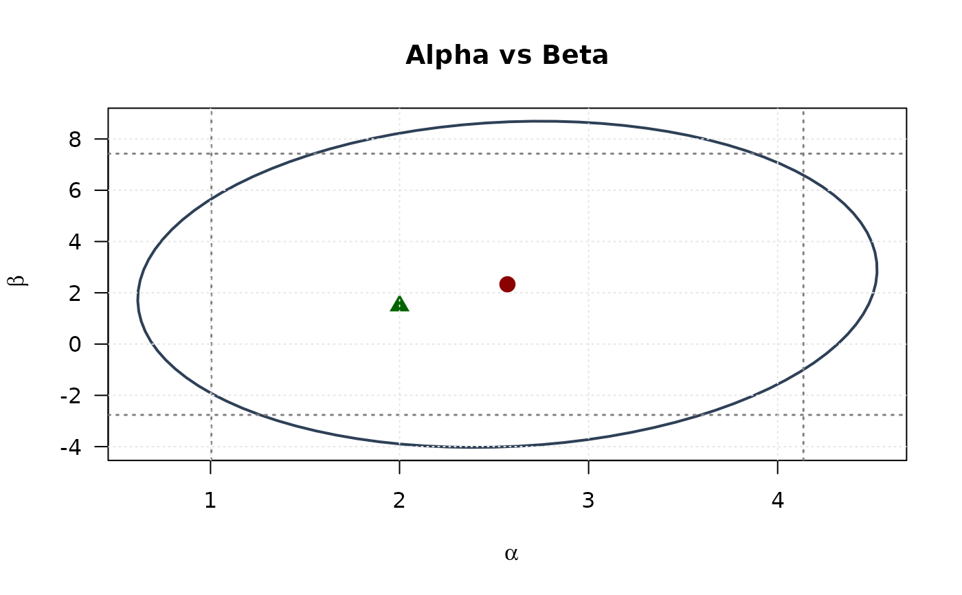
## Example 6: Confidence Ellipses (Selected pairs)

# Observed information
obs_info <- hsbkw(par = mle, data = data)
vcov_full <- solve(obs_info)

# Create confidence ellipses
theta <- seq(0, 2 * pi, length.out = 100)
chi2_val <- qchisq(0.95, df = 2)

# Alpha vs Beta ellipse
vcov_ab <- vcov_full[1:2, 1:2]
eig_decomp_ab <- eigen(vcov_ab)
ellipse_ab <- matrix(NA, nrow = 100, ncol = 2)
for (i in 1:100) {
  v <- c(cos(theta[i]), sin(theta[i]))
  ellipse_ab[i, ] <- mle[1:2] + sqrt(chi2_val) *
    (eig_decomp_ab$vectors %*% diag(sqrt(eig_decomp_ab$values)) %*% v)
}

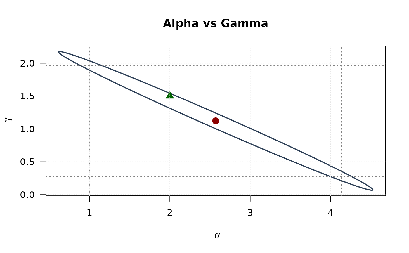
# Alpha vs Gamma ellipse
vcov_ag <- vcov_full[c(1, 3), c(1, 3)]
eig_decomp_ag <- eigen(vcov_ag)
ellipse_ag <- matrix(NA, nrow = 100, ncol = 2)
for (i in 1:100) {
  v <- c(cos(theta[i]), sin(theta[i]))
  ellipse_ag[i, ] <- mle[c(1, 3)] + sqrt(chi2_val) *
    (eig_decomp_ag$vectors %*% diag(sqrt(eig_decomp_ag$values)) %*% v)
}

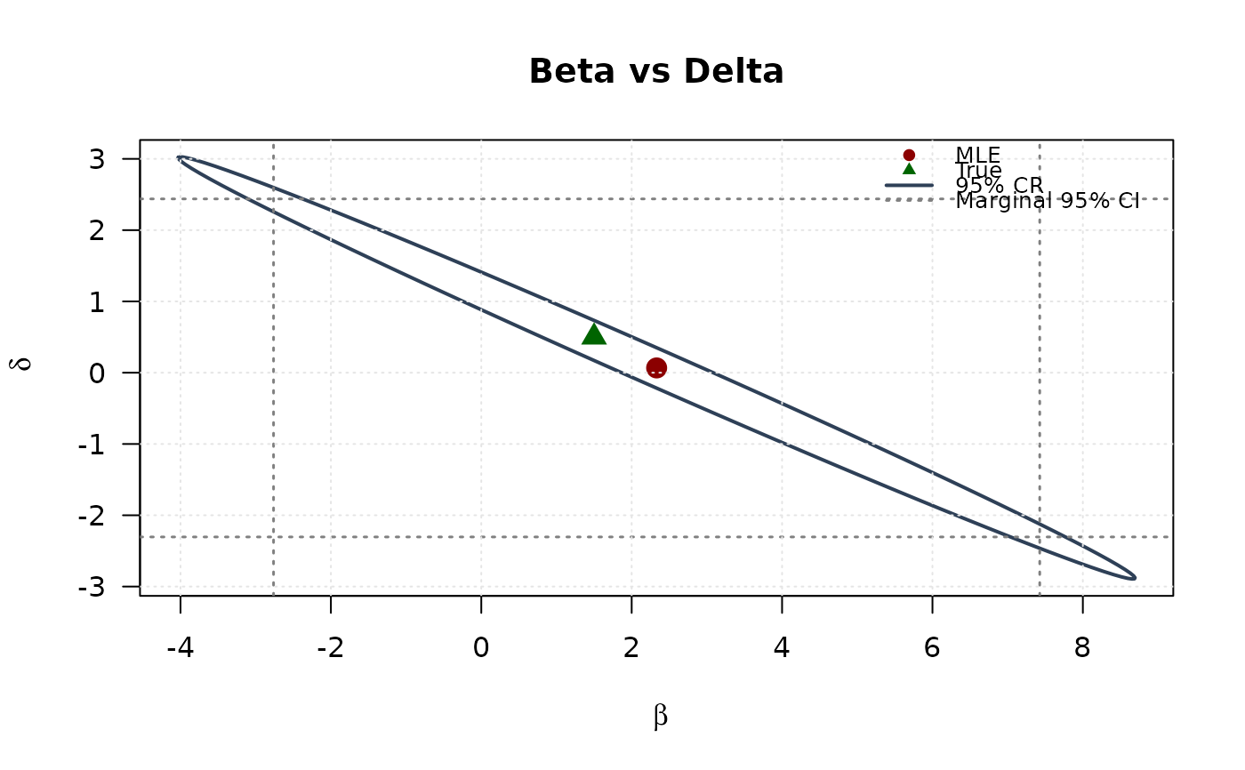
# Beta vs Delta ellipse
vcov_bd <- vcov_full[c(2, 4), c(2, 4)]
eig_decomp_bd <- eigen(vcov_bd)
ellipse_bd <- matrix(NA, nrow = 100, ncol = 2)
for (i in 1:100) {
  v <- c(cos(theta[i]), sin(theta[i]))
  ellipse_bd[i, ] <- mle[c(2, 4)] + sqrt(chi2_val) *
    (eig_decomp_bd$vectors %*% diag(sqrt(eig_decomp_bd$values)) %*% v)
}

# Marginal confidence intervals
se_ab <- sqrt(diag(vcov_ab))
ci_alpha_ab <- mle[1] + c(-1, 1) * 1.96 * se_ab[1]
ci_beta_ab <- mle[2] + c(-1, 1) * 1.96 * se_ab[2]

se_ag <- sqrt(diag(vcov_ag))
ci_alpha_ag <- mle[1] + c(-1, 1) * 1.96 * se_ag[1]
ci_gamma_ag <- mle[3] + c(-1, 1) * 1.96 * se_ag[2]

se_bd <- sqrt(diag(vcov_bd))
ci_beta_bd <- mle[2] + c(-1, 1) * 1.96 * se_bd[1]
ci_delta_bd <- mle[4] + c(-1, 1) * 1.96 * se_bd[2]

# Plot selected ellipses

# Alpha vs Beta
plot(ellipse_ab[, 1], ellipse_ab[, 2], type = "l", lwd = 2, col = "#2E4057",
     xlab = expression(alpha), ylab = expression(beta),
     main = "Alpha vs Beta", las = 1, xlim = range(ellipse_ab[, 1], ci_alpha_ab),
     ylim = range(ellipse_ab[, 2], ci_beta_ab))
abline(v = ci_alpha_ab, col = "#808080", lty = 3, lwd = 1.5)
abline(h = ci_beta_ab, col = "#808080", lty = 3, lwd = 1.5)
points(mle[1], mle[2], pch = 19, col = "#8B0000", cex = 1.5)
points(true_params[1], true_params[2], pch = 17, col = "#006400", cex = 1.5)
grid(col = "gray90")


# Alpha vs Gamma
plot(ellipse_ag[, 1], ellipse_ag[, 2], type = "l", lwd = 2, col = "#2E4057",
     xlab = expression(alpha), ylab = expression(gamma),
     main = "Alpha vs Gamma", las = 1, xlim = range(ellipse_ag[, 1], ci_alpha_ag),
     ylim = range(ellipse_ag[, 2], ci_gamma_ag))
abline(v = ci_alpha_ag, col = "#808080", lty = 3, lwd = 1.5)
abline(h = ci_gamma_ag, col = "#808080", lty = 3, lwd = 1.5)
points(mle[1], mle[3], pch = 19, col = "#8B0000", cex = 1.5)
points(true_params[1], true_params[3], pch = 17, col = "#006400", cex = 1.5)
grid(col = "gray90")


# Beta vs Delta
plot(ellipse_bd[, 1], ellipse_bd[, 2], type = "l", lwd = 2, col = "#2E4057",
     xlab = expression(beta), ylab = expression(delta),
     main = "Beta vs Delta", las = 1, xlim = range(ellipse_bd[, 1], ci_beta_bd),
     ylim = range(ellipse_bd[, 2], ci_delta_bd))
abline(v = ci_beta_bd, col = "#808080", lty = 3, lwd = 1.5)
abline(h = ci_delta_bd, col = "#808080", lty = 3, lwd = 1.5)
points(mle[2], mle[4], pch = 19, col = "#8B0000", cex = 1.5)
points(true_params[2], true_params[4], pch = 17, col = "#006400", cex = 1.5)
grid(col = "gray90")

legend("topright",
       legend = c("MLE", "True", "95% CR", "Marginal 95% CI"),
       col = c("#8B0000", "#006400", "#2E4057", "#808080"),
       pch = c(19, 17, NA, NA),
       lty = c(NA, NA, 1, 3),
       lwd = c(NA, NA, 2, 1.5),
       bty = "n", cex = 0.8)


# }