Random Number Generation for the McDonald (Mc)/Beta Power Distribution

Generates random deviates from the McDonald (Mc) distribution (also known as Beta Power) with parameters gamma (\(\gamma\)), delta (\(\delta\)), and lambda (\(\lambda\)). This distribution is a special case of the Generalized Kumaraswamy (GKw) distribution where \(\alpha = 1\) and \(\beta = 1\).

Usage

rmc(n, gamma, delta, lambda)

Arguments

n: Number of observations. If length(n) > 1, the length is taken to be the number required. Must be a non-negative integer.
gamma: Shape parameter gamma > 0. Can be a scalar or a vector. Default: 1.0.
delta: Shape parameter delta >= 0. Can be a scalar or a vector. Default: 0.0.
lambda: Shape parameter lambda > 0. Can be a scalar or a vector. Default: 1.0.

Value

A vector of length n containing random deviates from the Mc distribution, with values in (0, 1). The length of the result is determined by n and the recycling rule applied to the parameters (gamma, delta, lambda). Returns NaN if parameters are invalid (e.g., gamma <= 0, delta < 0, lambda <= 0).

Details

The generation method uses the relationship between the GKw distribution and the Beta distribution. The general procedure for GKw (rgkw) is: If \(W \sim \mathrm{Beta}(\gamma, \delta+1)\), then \(X = \{1 - [1 - W^{1/\lambda}]^{1/\beta}\}^{1/\alpha}\) follows the GKw(\(\alpha, \beta, \gamma, \delta, \lambda\)) distribution.

For the Mc distribution, \(\alpha=1\) and \(\beta=1\). Therefore, the algorithm simplifies significantly:

Generate \(U \sim \mathrm{Beta}(\gamma, \delta+1)\) using rbeta.
Compute the Mc variate \(X = U^{1/\lambda}\).

This procedure is implemented efficiently, handling parameter recycling as needed.

References

McDonald, J. B. (1984). Some generalized functions for the size distribution of income. Econometrica, 52(3), 647-663.

Cordeiro, G. M., & de Castro, M. (2011). A new family of generalized distributions. Journal of Statistical Computation and Simulation,

Kumaraswamy, P. (1980). A generalized probability density function for double-bounded random processes. Journal of Hydrology, 46(1-2), 79-88.

Devroye, L. (1986). Non-Uniform Random Variate Generation. Springer-Verlag. (General methods for random variate generation).

Author

Lopes, J. E.

Examples

# \donttest{
set.seed(2028) # for reproducibility

# Generate 1000 random values from a specific Mc distribution
gamma_par <- 2.0
delta_par <- 1.5
lambda_par <- 1.0 # Equivalent to Beta(gamma, delta+1)

x_sample_mc <- rmc(1000, gamma = gamma_par, delta = delta_par,
                   lambda = lambda_par)
summary(x_sample_mc)
#>    Min. 1st Qu.  Median    Mean 3rd Qu.    Max. 
#> 0.01013 0.27034 0.43516 0.44456 0.60679 0.97755 

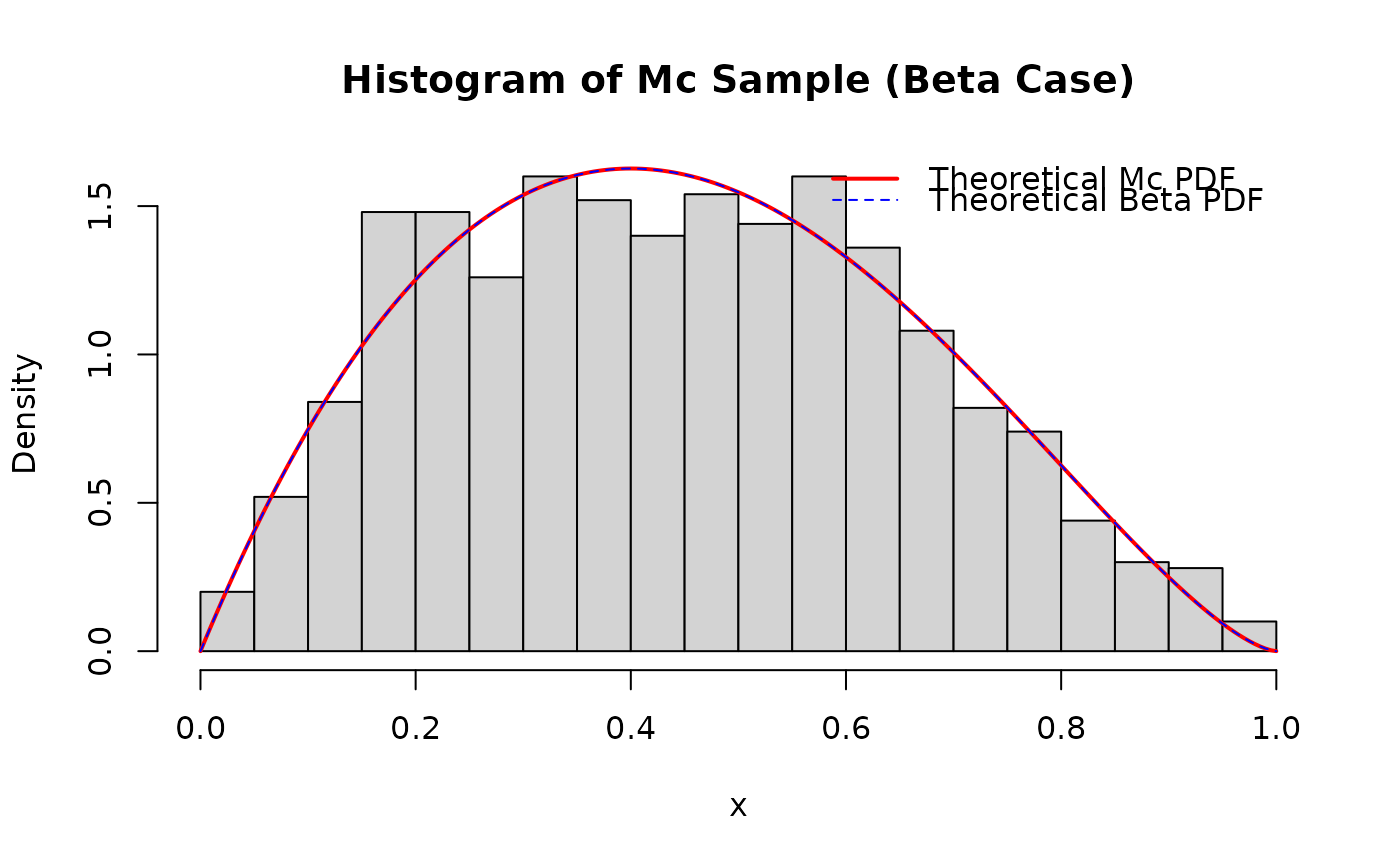
# Histogram of generated values compared to theoretical density
hist(x_sample_mc, breaks = 30, freq = FALSE, # freq=FALSE for density
     main = "Histogram of Mc Sample (Beta Case)", xlab = "x")
curve(dmc(x, gamma = gamma_par, delta = delta_par, lambda = lambda_par),
      add = TRUE, col = "red", lwd = 2, n = 201)
curve(stats::dbeta(x, gamma_par, delta_par + 1), add=TRUE, col="blue", lty=2)
legend("topright", legend = c("Theoretical Mc PDF", "Theoretical Beta PDF"),
       col = c("red", "blue"), lwd = c(2,1), lty=c(1,2), bty = "n")


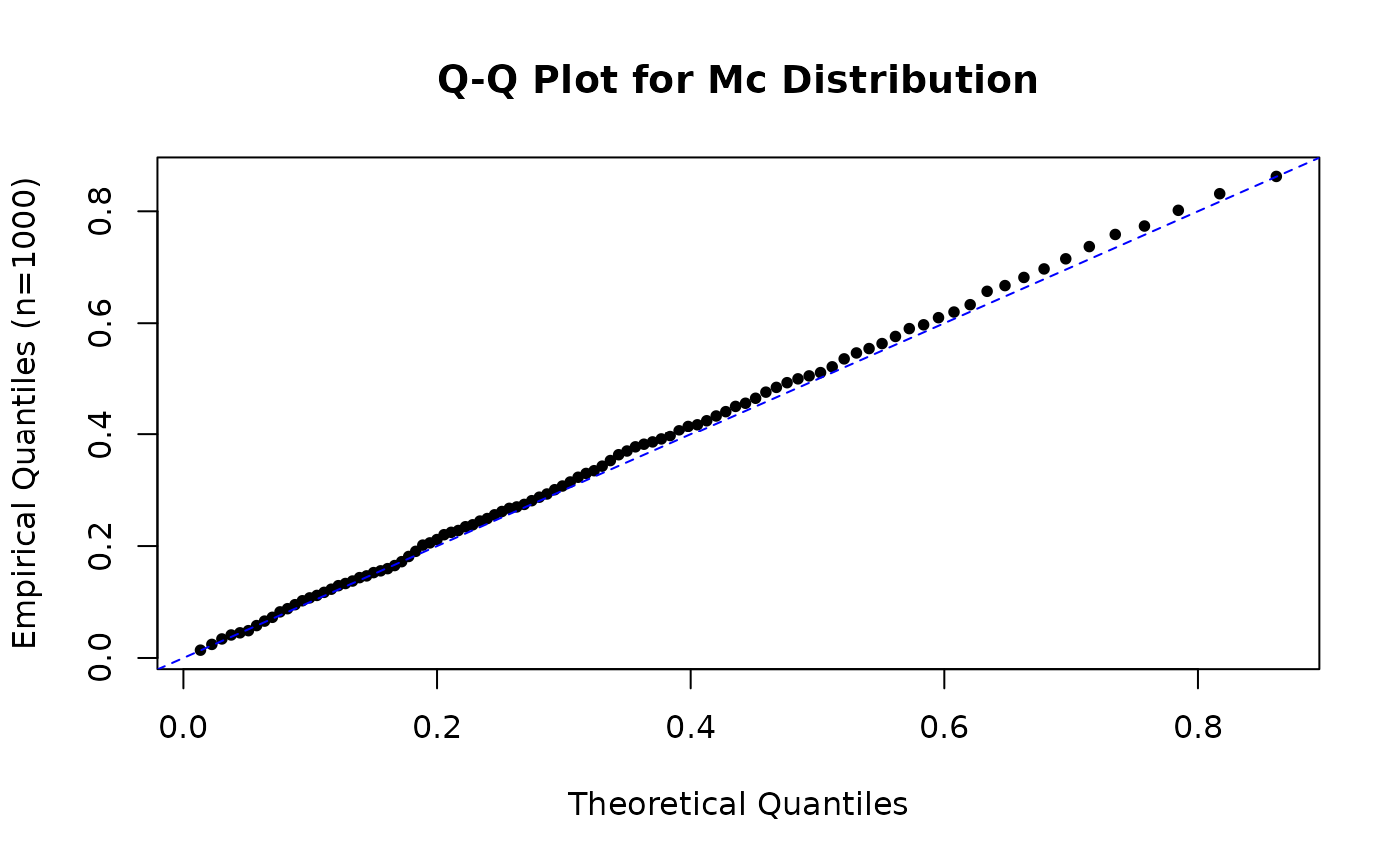
# Comparing empirical and theoretical quantiles (Q-Q plot)
lambda_par_qq <- 0.7 # Use lambda != 1 for non-Beta case
x_sample_mc_qq <- rmc(1000, gamma = gamma_par, delta = delta_par,
                      lambda = lambda_par_qq)
prob_points <- seq(0.01, 0.99, by = 0.01)
theo_quantiles <- qmc(prob_points, gamma = gamma_par, delta = delta_par,
                      lambda = lambda_par_qq)
emp_quantiles <- quantile(x_sample_mc_qq, prob_points, type = 7)

plot(theo_quantiles, emp_quantiles, pch = 16, cex = 0.8,
     main = "Q-Q Plot for Mc Distribution",
     xlab = "Theoretical Quantiles", ylab = "Empirical Quantiles (n=1000)")
abline(a = 0, b = 1, col = "blue", lty = 2)


# Compare summary stats with rgkw(..., alpha=1, beta=1, ...)
# Note: individual values will differ due to randomness
x_sample_gkw <- rgkw(1000, alpha = 1.0, beta = 1.0, gamma = gamma_par,
                     delta = delta_par, lambda = lambda_par_qq)
print("Summary stats for rmc sample:")
#> [1] "Summary stats for rmc sample:"
print(summary(x_sample_mc_qq))
#>      Min.   1st Qu.    Median      Mean   3rd Qu.      Max. 
#> 0.0008202 0.1596539 0.3145063 0.3473583 0.5006081 0.9639265 
print("Summary stats for rgkw(alpha=1, beta=1) sample:")
#> [1] "Summary stats for rgkw(alpha=1, beta=1) sample:"
print(summary(x_sample_gkw)) # Should be similar
#>     Min.  1st Qu.   Median     Mean  3rd Qu.     Max. 
#> 0.007415 0.159005 0.298210 0.330192 0.483725 0.932327 

# }