Density of the McDonald (Mc)/Beta Power Distribution Distribution

Computes the probability density function (PDF) for the McDonald (Mc) distribution (also previously referred to as Beta Power) with parameters gamma ($\gamma$), delta ($\delta$), and lambda ($\lambda$). This distribution is defined on the interval (0, 1).

Usage

dmc(x, gamma, delta, lambda, log_prob = FALSE)

Arguments

x: Vector of quantiles (values between 0 and 1).
gamma: Shape parameter gamma > 0. Can be a scalar or a vector. Default: 1.0.
delta: Shape parameter delta >= 0. Can be a scalar or a vector. Default: 0.0.
lambda: Shape parameter lambda > 0. Can be a scalar or a vector. Default: 1.0.
log_prob: Logical; if TRUE, the logarithm of the density is returned ($\log(f(x))$). Default: FALSE.

Value

A vector of density values ($f(x)$) or log-density values ($\log(f(x))$). The length of the result is determined by the recycling rule applied to the arguments (x, gamma, delta, lambda). Returns 0 (or -Inf if log_prob = TRUE) for x outside the interval (0, 1), or NaN if parameters are invalid (e.g., gamma <= 0, delta < 0, lambda <= 0).

Details

The probability density function (PDF) of the McDonald (Mc) distribution is given by: $$ f(x; \gamma, \delta, \lambda) = \frac{\lambda}{B(\gamma,\delta+1)} x^{\gamma \lambda - 1} (1 - x^\lambda)^\delta $$ for $0 < x < 1$, where $B(a,b)$ is the Beta function (beta).

The Mc distribution is a special case of the five-parameter Generalized Kumaraswamy (GKw) distribution (dgkw) obtained by setting the parameters $\alpha = 1$ and $\beta = 1$. It was introduced by McDonald (1984) and is related to the Generalized Beta distribution of the first kind (GB1). When $\lambda=1$, it simplifies to the standard Beta distribution with parameters $\gamma$ and $\delta+1$.

References

McDonald, J. B. (1984). Some generalized functions for the size distribution of income. Econometrica, 52(3), 647-663.

Cordeiro, G. M., & de Castro, M. (2011). A new family of generalized distributions. Journal of Statistical Computation and Simulation,

Kumaraswamy, P. (1980). A generalized probability density function for double-bounded random processes. Journal of Hydrology, 46(1-2), 79-88.

Author

Lopes, J. E.

Examples

# \donttest{
# Example values
x_vals <- c(0.2, 0.5, 0.8)
gamma_par <- 2.0
delta_par <- 1.5
lambda_par <- 1.0 # Equivalent to Beta(gamma, delta+1)

# Calculate density using dmc
densities <- dmc(x_vals, gamma_par, delta_par, lambda_par)
print(densities)
#> [1] 1.252198 1.546796 0.626099
# Compare with Beta density
print(stats::dbeta(x_vals, shape1 = gamma_par, shape2 = delta_par + 1))
#> [1] 1.252198 1.546796 0.626099

# Calculate log-density
log_densities <- dmc(x_vals, gamma_par, delta_par, lambda_par, log_prob = TRUE)
print(log_densities)
#> [1]  0.2249005  0.4361857 -0.4682467

# Compare with dgkw setting alpha = 1, beta = 1
densities_gkw <- dgkw(x_vals, alpha = 1.0, beta = 1.0, gamma = gamma_par,
                      delta = delta_par, lambda = lambda_par)
print(paste("Max difference:", max(abs(densities - densities_gkw)))) # Should be near zero
#> [1] "Max difference: 0"

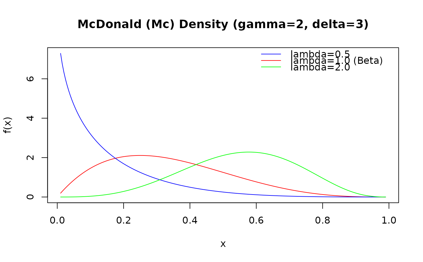
# Plot the density for different lambda values
curve_x <- seq(0.01, 0.99, length.out = 200)
curve_y1 <- dmc(curve_x, gamma = 2, delta = 3, lambda = 0.5)
curve_y2 <- dmc(curve_x, gamma = 2, delta = 3, lambda = 1.0) # Beta(2, 4)
curve_y3 <- dmc(curve_x, gamma = 2, delta = 3, lambda = 2.0)

plot(curve_x, curve_y2, type = "l", main = "McDonald (Mc) Density (gamma=2, delta=3)",
     xlab = "x", ylab = "f(x)", col = "red", ylim = range(0, curve_y1, curve_y2, curve_y3))
lines(curve_x, curve_y1, col = "blue")
lines(curve_x, curve_y3, col = "green")
legend("topright", legend = c("lambda=0.5", "lambda=1.0 (Beta)", "lambda=2.0"),
       col = c("blue", "red", "green"), lty = 1, bty = "n")

# }