Random Generation for the Beta Distribution (gamma, delta+1 Parameterization)

Generates random deviates from the standard Beta distribution, using a parameterization common in generalized distribution families. The distribution is parameterized by gamma (\(\gamma\)) and delta (\(\delta\)), corresponding to the standard Beta distribution with shape parameters shape1 = gamma and shape2 = delta + 1. This is a special case of the Generalized Kumaraswamy (GKw) distribution where \(\alpha = 1\), \(\beta = 1\), and \(\lambda = 1\).

Usage

rbeta_(n, gamma, delta)

Arguments

n: Number of observations. If length(n) > 1, the length is taken to be the number required. Must be a non-negative integer.
gamma: First shape parameter (shape1), \(\gamma > 0\). Can be a scalar or a vector. Default: 1.0.
delta: Second shape parameter is delta + 1 (shape2), requires \(\delta \ge 0\) so that shape2 >= 1. Can be a scalar or a vector. Default: 0.0 (leading to shape2 = 1, i.e., Uniform).

Value

A numeric vector of length n containing random deviates from the Beta(\(\gamma, \delta+1\)) distribution, with values in (0, 1). The length of the result is determined by n and the recycling rule applied to the parameters (gamma, delta). Returns NaN if parameters are invalid (e.g., gamma <= 0, delta < 0).

Details

This function generates samples from a Beta distribution with parameters shape1 = gamma and shape2 = delta + 1. It is equivalent to calling stats::rbeta(n, shape1 = gamma, shape2 = delta + 1).

This distribution arises as a special case of the five-parameter Generalized Kumaraswamy (GKw) distribution (rgkw) obtained by setting \(\alpha = 1\), \(\beta = 1\), and \(\lambda = 1\). It is therefore also equivalent to the McDonald (Mc)/Beta Power distribution (rmc) with \(\lambda = 1\).

The function likely calls R's underlying rbeta function but ensures consistent parameter recycling and handling within the C++ environment, matching the style of other functions in the related families.

References

Johnson, N. L., Kotz, S., & Balakrishnan, N. (1995). Continuous Univariate Distributions, Volume 2 (2nd ed.). Wiley.

Cordeiro, G. M., & de Castro, M. (2011). A new family of generalized distributions. Journal of Statistical Computation and Simulation,

Devroye, L. (1986). Non-Uniform Random Variate Generation. Springer-Verlag.

Author

Lopes, J. E.

Examples

# \donttest{
set.seed(2030) # for reproducibility

# Generate 1000 samples using rbeta_
gamma_par <- 2.0 # Corresponds to shape1
delta_par <- 3.0 # Corresponds to shape2 - 1
shape1 <- gamma_par
shape2 <- delta_par + 1

x_sample <- rbeta_(1000, gamma = gamma_par, delta = delta_par)
summary(x_sample)
#>     Min.  1st Qu.   Median     Mean  3rd Qu.     Max. 
#> 0.007135 0.190328 0.306978 0.335931 0.466661 0.886553 

# Compare with stats::rbeta
x_sample_stats <- stats::rbeta(1000, shape1 = shape1, shape2 = shape2)
# Visually compare histograms or QQ-plots
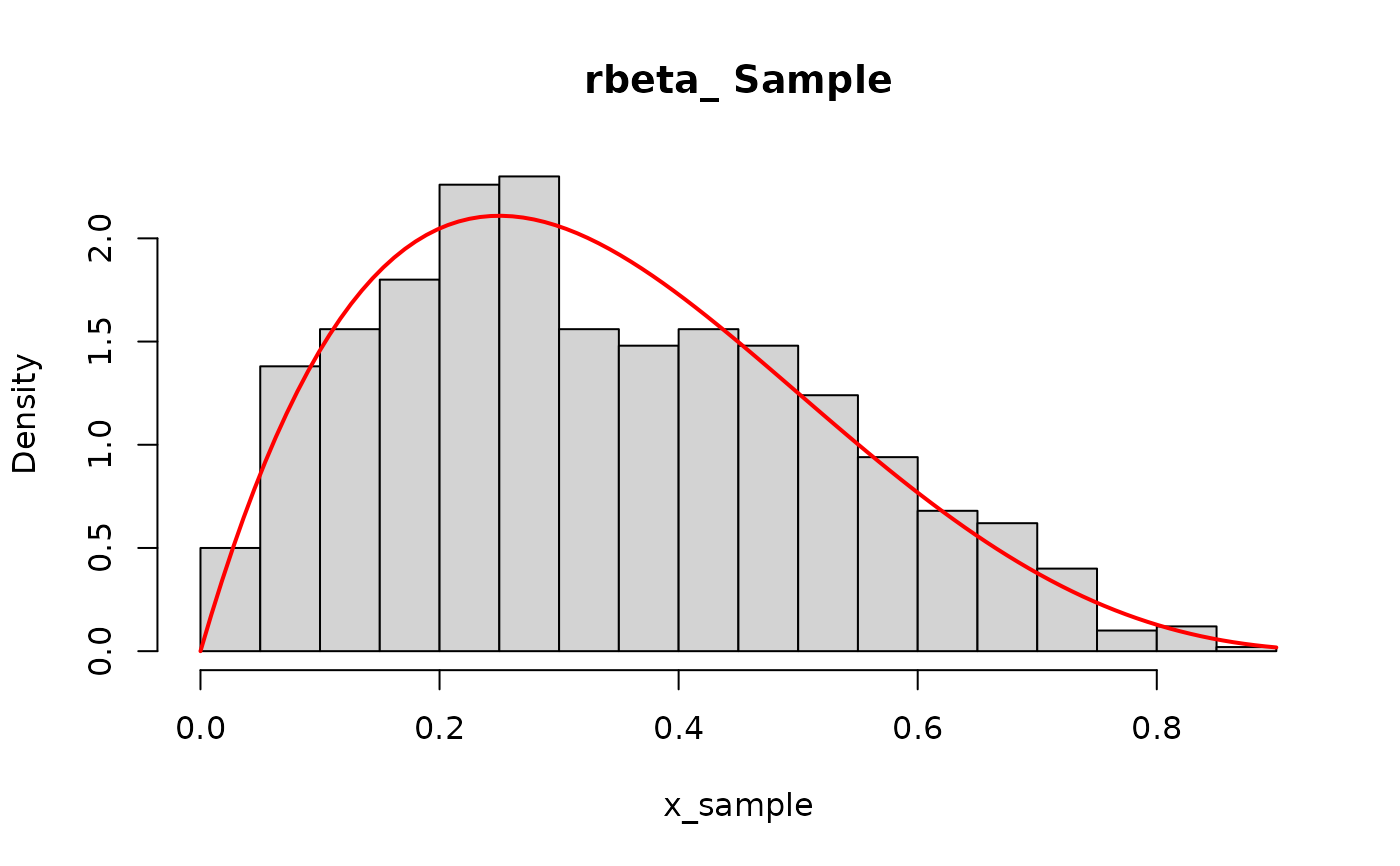
hist(x_sample, main="rbeta_ Sample", freq=FALSE, breaks=30)
curve(dbeta_(x, gamma_par, delta_par), add=TRUE, col="red", lwd=2)

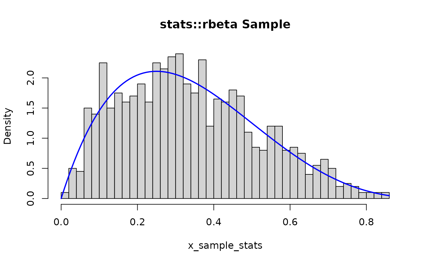
hist(x_sample_stats, main="stats::rbeta Sample", freq=FALSE, breaks=30)
curve(stats::dbeta(x, shape1, shape2), add=TRUE, col="blue", lwd=2)

# Compare summary stats (should be similar due to randomness)
print(summary(x_sample))
#>     Min.  1st Qu.   Median     Mean  3rd Qu.     Max. 
#> 0.007135 0.190328 0.306978 0.335931 0.466661 0.886553 
print(summary(x_sample_stats))
#>    Min. 1st Qu.  Median    Mean 3rd Qu.    Max. 
#> 0.01034 0.19696 0.31440 0.33723 0.45535 0.84423 

# Compare summary stats with rgkw(alpha=1, beta=1, lambda=1)
x_sample_gkw <- rgkw(1000, alpha = 1.0, beta = 1.0, gamma = gamma_par,
                     delta = delta_par, lambda = 1.0)
print("Summary stats for rgkw(a=1,b=1,l=1) sample:")
#> [1] "Summary stats for rgkw(a=1,b=1,l=1) sample:"
print(summary(x_sample_gkw))
#>     Min.  1st Qu.   Median     Mean  3rd Qu.     Max. 
#> 0.004943 0.189179 0.313707 0.328485 0.445345 0.892626 

# Compare summary stats with rmc(lambda=1)
x_sample_mc <- rmc(1000, gamma = gamma_par, delta = delta_par, lambda = 1.0)
print("Summary stats for rmc(l=1) sample:")
#> [1] "Summary stats for rmc(l=1) sample:"
print(summary(x_sample_mc))
#>    Min. 1st Qu.  Median    Mean 3rd Qu.    Max. 
#> 0.00105 0.19221 0.31254 0.33300 0.45504 0.91894 

# }