Density of the Beta Distribution (gamma, delta+1 Parameterization)

Computes the probability density function (PDF) for the standard Beta distribution, using a parameterization common in generalized distribution families. The distribution is parameterized by gamma ($\gamma$) and delta ($\delta$), corresponding to the standard Beta distribution with shape parameters shape1 = gamma and shape2 = delta + 1. The distribution is defined on the interval (0, 1).

Usage

dbeta_(x, gamma, delta, log_prob = FALSE)

Arguments

x: Vector of quantiles (values between 0 and 1).
gamma: First shape parameter (shape1), $\gamma > 0$. Can be a scalar or a vector. Default: 1.0.
delta: Second shape parameter is delta + 1 (shape2), requires $\delta \ge 0$ so that shape2 >= 1. Can be a scalar or a vector. Default: 0.0 (leading to shape2 = 1).
log_prob: Logical; if TRUE, the logarithm of the density is returned ($\log(f(x))$). Default: FALSE.

Value

A vector of density values ($f(x)$) or log-density values ($\log(f(x))$). The length of the result is determined by the recycling rule applied to the arguments (x, gamma, delta). Returns 0 (or -Inf if log_prob = TRUE) for x outside the interval (0, 1), or NaN if parameters are invalid (e.g., gamma <= 0, delta < 0).

Details

The probability density function (PDF) calculated by this function corresponds to a standard Beta distribution $Beta(\gamma, \delta+1)$: $$ f(x; \gamma, \delta) = \frac{x^{\gamma-1} (1-x)^{(\delta+1)-1}}{B(\gamma, \delta+1)} = \frac{x^{\gamma-1} (1-x)^{\delta}}{B(\gamma, \delta+1)} $$ for $0 < x < 1$, where $B(a,b)$ is the Beta function (beta).

This specific parameterization arises as a special case of the five-parameter Generalized Kumaraswamy (GKw) distribution (dgkw) obtained by setting the parameters $\alpha = 1$, $\beta = 1$, and $\lambda = 1$. It is therefore equivalent to the McDonald (Mc)/Beta Power distribution (dmc) with $\lambda = 1$.

Note the difference in the second parameter compared to dbeta, where dbeta(x, shape1, shape2) uses shape2 directly. Here, shape1 = gamma and shape2 = delta + 1.

References

Johnson, N. L., Kotz, S., & Balakrishnan, N. (1995). Continuous Univariate Distributions, Volume 2 (2nd ed.). Wiley.

Cordeiro, G. M., & de Castro, M. (2011). A new family of generalized distributions. Journal of Statistical Computation and Simulation,

Author

Lopes, J. E.

Examples

# \donttest{
# Example values
x_vals <- c(0.2, 0.5, 0.8)
gamma_par <- 2.0 # Corresponds to shape1
delta_par <- 3.0 # Corresponds to shape2 - 1
shape1 <- gamma_par
shape2 <- delta_par + 1

# Calculate density using dbeta_
densities <- dbeta_(x_vals, gamma_par, delta_par)
print(densities)
#> [1] 2.048 1.250 0.128

# Compare with stats::dbeta
densities_stats <- stats::dbeta(x_vals, shape1 = shape1, shape2 = shape2)
print(paste("Max difference vs stats::dbeta:", max(abs(densities - densities_stats))))
#> [1] "Max difference vs stats::dbeta: 0"

# Compare with dgkw setting alpha=1, beta=1, lambda=1
densities_gkw <- dgkw(x_vals, alpha = 1.0, beta = 1.0, gamma = gamma_par,
                      delta = delta_par, lambda = 1.0)
print(paste("Max difference vs dgkw:", max(abs(densities - densities_gkw))))
#> [1] "Max difference vs dgkw: 0"

# Compare with dmc setting lambda=1
densities_mc <- dmc(x_vals, gamma = gamma_par, delta = delta_par, lambda = 1.0)
print(paste("Max difference vs dmc:", max(abs(densities - densities_mc))))
#> [1] "Max difference vs dmc: 4.44089209850063e-16"

# Calculate log-density
log_densities <- dbeta_(x_vals, gamma_par, delta_par, log_prob = TRUE)
print(log_densities)
#> [1]  0.7168637  0.2231436 -2.0557250
print(stats::dbeta(x_vals, shape1 = shape1, shape2 = shape2, log = TRUE))
#> [1]  0.7168637  0.2231436 -2.0557250

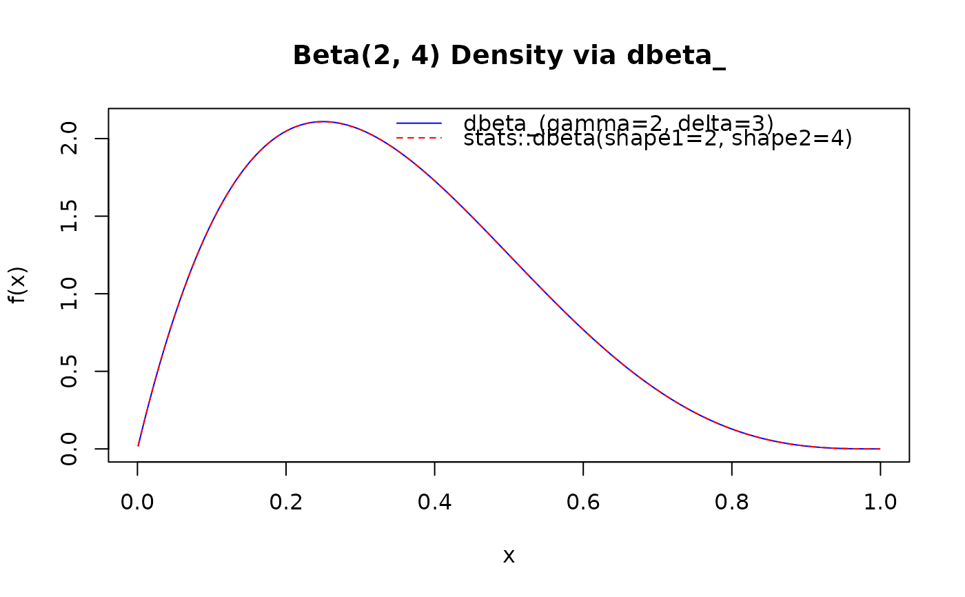
# Plot the density
curve_x <- seq(0.001, 0.999, length.out = 200)
curve_y <- dbeta_(curve_x, gamma = 2, delta = 3) # Beta(2, 4)
plot(curve_x, curve_y, type = "l", main = "Beta(2, 4) Density via dbeta_",
     xlab = "x", ylab = "f(x)", col = "blue")
curve(stats::dbeta(x, 2, 4), add=TRUE, col="red", lty=2)
legend("topright", legend=c("dbeta_(gamma=2, delta=3)", "stats::dbeta(shape1=2, shape2=4)"),
       col=c("blue", "red"), lty=c(1,2), bty="n")


# }