Negative Log-Likelihood for the Beta Distribution (gamma, delta+1 Parameterization)
Source:R/beta.R
llbeta.RdComputes the negative log-likelihood function for the standard Beta
distribution, using a parameterization common in generalized distribution
families. The distribution is parameterized by gamma (\(\gamma\)) and
delta (\(\delta\)), corresponding to the standard Beta distribution
with shape parameters shape1 = gamma and shape2 = delta + 1.
This function is suitable for maximum likelihood estimation.
Value
Returns a single double value representing the negative
log-likelihood (\(-\ell(\theta|\mathbf{x})\)). Returns Inf
if any parameter values in par are invalid according to their
constraints, or if any value in data is not in the interval (0, 1).
Details
This function calculates the negative log-likelihood for a Beta distribution
with parameters shape1 = gamma (\(\gamma\)) and shape2 = delta + 1 (\(\delta+1\)).
The probability density function (PDF) is:
$$
f(x | \gamma, \delta) = \frac{x^{\gamma-1} (1-x)^{\delta}}{B(\gamma, \delta+1)}
$$
for \(0 < x < 1\), where \(B(a,b)\) is the Beta function (beta).
The log-likelihood function \(\ell(\theta | \mathbf{x})\) for a sample
\(\mathbf{x} = (x_1, \dots, x_n)\) is \(\sum_{i=1}^n \ln f(x_i | \theta)\):
$$
\ell(\theta | \mathbf{x}) = \sum_{i=1}^{n} [(\gamma-1)\ln(x_i) + \delta\ln(1-x_i)] - n \ln B(\gamma, \delta+1)
$$
where \(\theta = (\gamma, \delta)\).
This function computes and returns the negative log-likelihood, \(-\ell(\theta|\mathbf{x})\),
suitable for minimization using optimization routines like optim.
It is equivalent to the negative log-likelihood of the GKw distribution
(llgkw) evaluated at \(\alpha=1, \beta=1, \lambda=1\), and also
to the negative log-likelihood of the McDonald distribution (llmc)
evaluated at \(\lambda=1\). The term \(\ln B(\gamma, \delta+1)\) is typically
computed using log-gamma functions (lgamma) for numerical stability.
References
Johnson, N. L., Kotz, S., & Balakrishnan, N. (1995). Continuous Univariate Distributions, Volume 2 (2nd ed.). Wiley.
Cordeiro, G. M., & de Castro, M. (2011). A new family of generalized distributions. Journal of Statistical Computation and Simulation,
Examples
# \donttest{
## Example 1: Basic Log-Likelihood Evaluation
# Generate sample data
set.seed(123)
n <- 1000
true_params <- c(gamma = 2.0, delta = 3.0)
data <- rbeta_(n, gamma = true_params[1], delta = true_params[2])
# Evaluate negative log-likelihood at true parameters
nll_true <- llbeta(par = true_params, data = data)
cat("Negative log-likelihood at true parameters:", nll_true, "\n")
#> Negative log-likelihood at true parameters: -359.6415
# Evaluate at different parameter values
test_params <- rbind(
c(1.5, 2.5),
c(2.0, 3.0),
c(2.5, 3.5)
)
nll_values <- apply(test_params, 1, function(p) llbeta(p, data))
results <- data.frame(
Gamma = test_params[, 1],
Delta = test_params[, 2],
NegLogLik = nll_values
)
print(results, digits = 4)
#> Gamma Delta NegLogLik
#> 1 1.5 2.5 -324.4
#> 2 2.0 3.0 -359.6
#> 3 2.5 3.5 -342.2
## Example 2: Maximum Likelihood Estimation
# Optimization using L-BFGS-B with bounds
fit <- optim(
par = c(1.5, 2.5),
fn = llbeta,
gr = grbeta,
data = data,
method = "L-BFGS-B",
lower = c(0.01, 0.01),
upper = c(100, 100),
hessian = TRUE
)
mle <- fit$par
names(mle) <- c("gamma", "delta")
se <- sqrt(diag(solve(fit$hessian)))
results <- data.frame(
Parameter = c("gamma", "delta"),
True = true_params,
MLE = mle,
SE = se,
CI_Lower = mle - 1.96 * se,
CI_Upper = mle + 1.96 * se
)
print(results, digits = 4)
#> Parameter True MLE SE CI_Lower CI_Upper
#> gamma gamma 2 2.029 0.08495 1.862 2.195
#> delta delta 3 2.997 0.17769 2.649 3.346
cat(sprintf(
"\nMLE corresponds approx to Beta(%.2f, %.2f)\n",
mle[1], mle[2] + 1
))
#>
#> MLE corresponds approx to Beta(2.03, 4.00)
cat(
"True corresponds to Beta(%.2f, %.2f)\n",
true_params[1], true_params[2] + 1
)
#> True corresponds to Beta(%.2f, %.2f)
#> 2 4
cat("\nNegative log-likelihood at MLE:", fit$value, "\n")
#>
#> Negative log-likelihood at MLE: -359.8439
cat("AIC:", 2 * fit$value + 2 * length(mle), "\n")
#> AIC: -715.6878
cat("BIC:", 2 * fit$value + length(mle) * log(n), "\n")
#> BIC: -705.8723
## Example 3: Comparing Optimization Methods
methods <- c("BFGS", "L-BFGS-B", "Nelder-Mead", "CG")
start_params <- c(1.5, 2.5)
comparison <- data.frame(
Method = character(),
Gamma = numeric(),
Delta = numeric(),
NegLogLik = numeric(),
Convergence = integer(),
stringsAsFactors = FALSE
)
for (method in methods) {
if (method %in% c("BFGS", "CG")) {
fit_temp <- optim(
par = start_params,
fn = llbeta,
gr = grbeta,
data = data,
method = method
)
} else if (method == "L-BFGS-B") {
fit_temp <- optim(
par = start_params,
fn = llbeta,
gr = grbeta,
data = data,
method = method,
lower = c(0.01, 0.01),
upper = c(100, 100)
)
} else {
fit_temp <- optim(
par = start_params,
fn = llbeta,
data = data,
method = method
)
}
comparison <- rbind(comparison, data.frame(
Method = method,
Gamma = fit_temp$par[1],
Delta = fit_temp$par[2],
NegLogLik = fit_temp$value,
Convergence = fit_temp$convergence,
stringsAsFactors = FALSE
))
}
print(comparison, digits = 4, row.names = FALSE)
#> Method Gamma Delta NegLogLik Convergence
#> BFGS 2.029 2.997 -359.8 0
#> L-BFGS-B 2.029 2.997 -359.8 0
#> Nelder-Mead 2.029 2.997 -359.8 0
#> CG 2.029 2.997 -359.8 0
## Example 4: Likelihood Ratio Test
# Test H0: delta = 3 vs H1: delta free
loglik_full <- -fit$value
restricted_ll <- function(params_restricted, data, delta_fixed) {
llbeta(par = c(params_restricted[1], delta_fixed), data = data)
}
fit_restricted <- optim(
par = mle[1],
fn = restricted_ll,
data = data,
delta_fixed = 3,
method = "BFGS"
)
loglik_restricted <- -fit_restricted$value
lr_stat <- 2 * (loglik_full - loglik_restricted)
p_value <- pchisq(lr_stat, df = 1, lower.tail = FALSE)
cat("LR Statistic:", round(lr_stat, 4), "\n")
#> LR Statistic: 2e-04
cat("P-value:", format.pval(p_value, digits = 4), "\n")
#> P-value: 0.9884
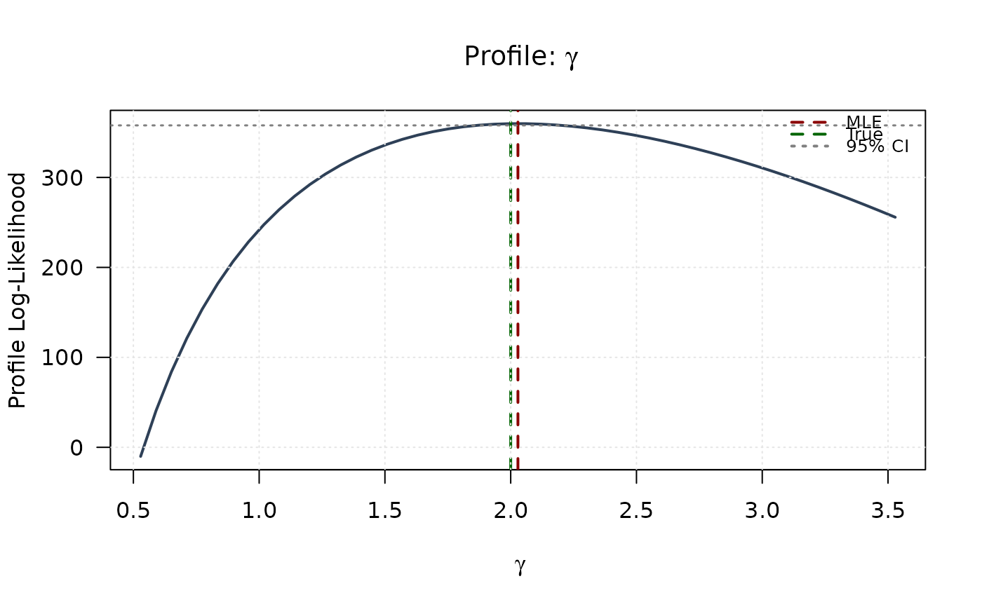
## Example 5: Univariate Profile Likelihoods
# Profile for gamma
gamma_grid <- seq(mle[1] - 1.5, mle[1] + 1.5, length.out = 50)
gamma_grid <- gamma_grid[gamma_grid > 0]
profile_ll_gamma <- numeric(length(gamma_grid))
for (i in seq_along(gamma_grid)) {
profile_fit <- optim(
par = mle[2],
fn = function(p) llbeta(c(gamma_grid[i], p), data),
method = "BFGS"
)
profile_ll_gamma[i] <- -profile_fit$value
}
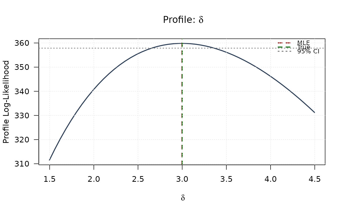
# Profile for delta
delta_grid <- seq(mle[2] - 1.5, mle[2] + 1.5, length.out = 50)
delta_grid <- delta_grid[delta_grid > 0]
profile_ll_delta <- numeric(length(delta_grid))
for (i in seq_along(delta_grid)) {
profile_fit <- optim(
par = mle[1],
fn = function(p) llbeta(c(p, delta_grid[i]), data),
method = "BFGS"
)
profile_ll_delta[i] <- -profile_fit$value
}
# 95% confidence threshold
chi_crit <- qchisq(0.95, df = 1)
threshold <- max(profile_ll_gamma) - chi_crit / 2
# Plot
plot(gamma_grid, profile_ll_gamma,
type = "l", lwd = 2, col = "#2E4057",
xlab = expression(gamma), ylab = "Profile Log-Likelihood",
main = expression(paste("Profile: ", gamma)), las = 1
)
abline(v = mle[1], col = "#8B0000", lty = 2, lwd = 2)
abline(v = true_params[1], col = "#006400", lty = 2, lwd = 2)
abline(h = threshold, col = "#808080", lty = 3, lwd = 1.5)
legend("topright",
legend = c("MLE", "True", "95% CI"),
col = c("#8B0000", "#006400", "#808080"),
lty = c(2, 2, 3), lwd = 2, bty = "n", cex = 0.8
)
grid(col = "gray90")
 plot(delta_grid, profile_ll_delta,
type = "l", lwd = 2, col = "#2E4057",
xlab = expression(delta), ylab = "Profile Log-Likelihood",
main = expression(paste("Profile: ", delta)), las = 1
)
abline(v = mle[2], col = "#8B0000", lty = 2, lwd = 2)
abline(v = true_params[2], col = "#006400", lty = 2, lwd = 2)
abline(h = threshold, col = "#808080", lty = 3, lwd = 1.5)
legend("topright",
legend = c("MLE", "True", "95% CI"),
col = c("#8B0000", "#006400", "#808080"),
lty = c(2, 2, 3), lwd = 2, bty = "n", cex = 0.8
)
grid(col = "gray90")
plot(delta_grid, profile_ll_delta,
type = "l", lwd = 2, col = "#2E4057",
xlab = expression(delta), ylab = "Profile Log-Likelihood",
main = expression(paste("Profile: ", delta)), las = 1
)
abline(v = mle[2], col = "#8B0000", lty = 2, lwd = 2)
abline(v = true_params[2], col = "#006400", lty = 2, lwd = 2)
abline(h = threshold, col = "#808080", lty = 3, lwd = 1.5)
legend("topright",
legend = c("MLE", "True", "95% CI"),
col = c("#8B0000", "#006400", "#808080"),
lty = c(2, 2, 3), lwd = 2, bty = "n", cex = 0.8
)
grid(col = "gray90")
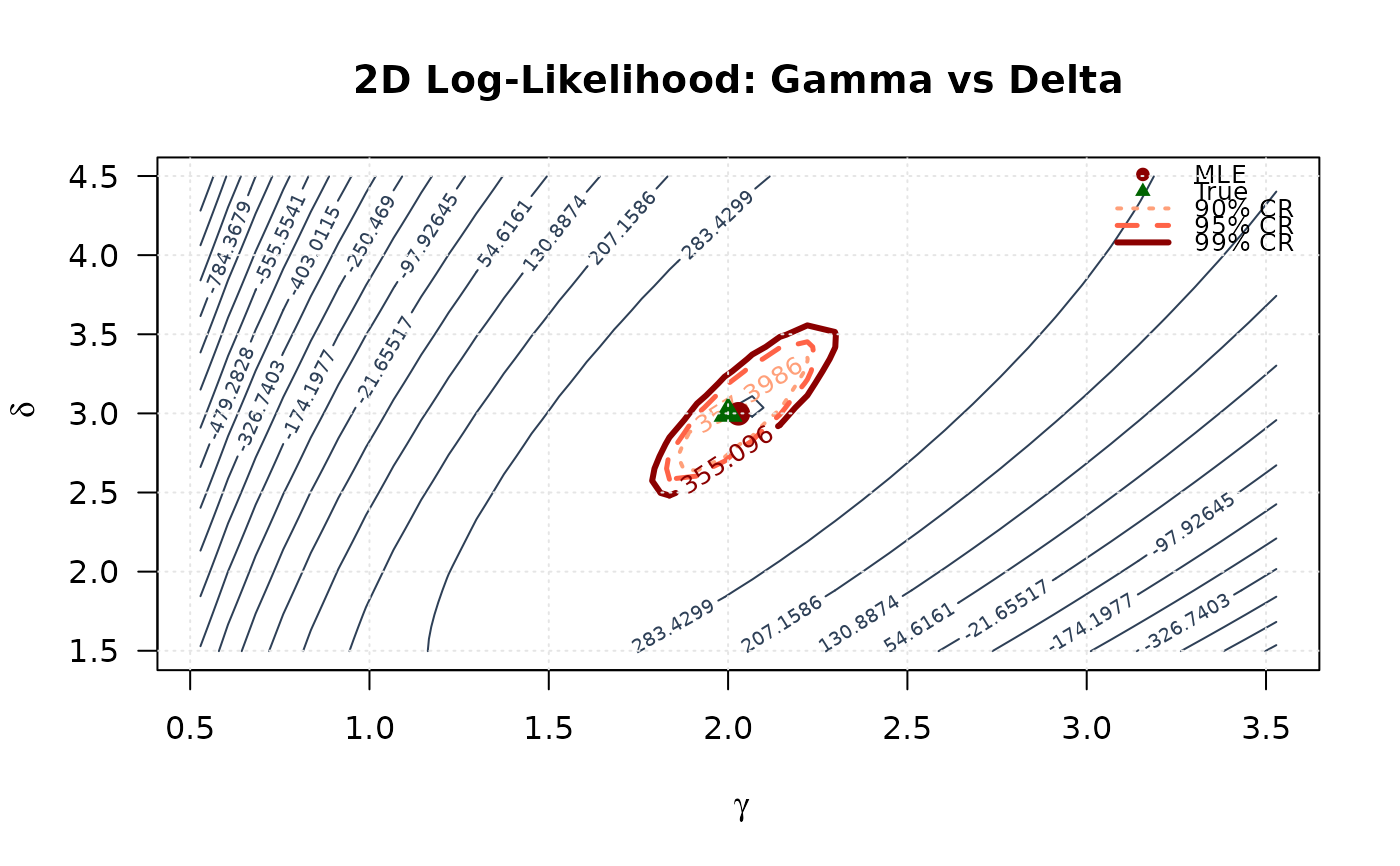
 ## Example 6: 2D Log-Likelihood Surface (Gamma vs Delta)
# Create 2D grid with wider range (±1.5)
gamma_2d <- seq(mle[1] - 1.5, mle[1] + 1.5, length.out = round(n / 25))
delta_2d <- seq(mle[2] - 1.5, mle[2] + 1.5, length.out = round(n / 25))
gamma_2d <- gamma_2d[gamma_2d > 0]
delta_2d <- delta_2d[delta_2d > 0]
# Compute log-likelihood surface
ll_surface_gd <- matrix(NA, nrow = length(gamma_2d), ncol = length(delta_2d))
for (i in seq_along(gamma_2d)) {
for (j in seq_along(delta_2d)) {
ll_surface_gd[i, j] <- -llbeta(c(gamma_2d[i], delta_2d[j]), data)
}
}
# Confidence region levels
max_ll_gd <- max(ll_surface_gd, na.rm = TRUE)
levels_90_gd <- max_ll_gd - qchisq(0.90, df = 2) / 2
levels_95_gd <- max_ll_gd - qchisq(0.95, df = 2) / 2
levels_99_gd <- max_ll_gd - qchisq(0.99, df = 2) / 2
# Plot contour
contour(gamma_2d, delta_2d, ll_surface_gd,
xlab = expression(gamma), ylab = expression(delta),
main = "2D Log-Likelihood: Gamma vs Delta",
levels = seq(min(ll_surface_gd, na.rm = TRUE), max_ll_gd, length.out = 20),
col = "#2E4057", las = 1, lwd = 1
)
contour(gamma_2d, delta_2d, ll_surface_gd,
levels = c(levels_90_gd, levels_95_gd, levels_99_gd),
col = c("#FFA07A", "#FF6347", "#8B0000"),
lwd = c(2, 2.5, 3), lty = c(3, 2, 1),
add = TRUE, labcex = 0.8
)
points(mle[1], mle[2], pch = 19, col = "#8B0000", cex = 1.5)
points(true_params[1], true_params[2], pch = 17, col = "#006400", cex = 1.5)
legend("topright",
legend = c("MLE", "True", "90% CR", "95% CR", "99% CR"),
col = c("#8B0000", "#006400", "#FFA07A", "#FF6347", "#8B0000"),
pch = c(19, 17, NA, NA, NA),
lty = c(NA, NA, 3, 2, 1),
lwd = c(NA, NA, 2, 2.5, 3),
bty = "n", cex = 0.8
)
grid(col = "gray90")
## Example 6: 2D Log-Likelihood Surface (Gamma vs Delta)
# Create 2D grid with wider range (±1.5)
gamma_2d <- seq(mle[1] - 1.5, mle[1] + 1.5, length.out = round(n / 25))
delta_2d <- seq(mle[2] - 1.5, mle[2] + 1.5, length.out = round(n / 25))
gamma_2d <- gamma_2d[gamma_2d > 0]
delta_2d <- delta_2d[delta_2d > 0]
# Compute log-likelihood surface
ll_surface_gd <- matrix(NA, nrow = length(gamma_2d), ncol = length(delta_2d))
for (i in seq_along(gamma_2d)) {
for (j in seq_along(delta_2d)) {
ll_surface_gd[i, j] <- -llbeta(c(gamma_2d[i], delta_2d[j]), data)
}
}
# Confidence region levels
max_ll_gd <- max(ll_surface_gd, na.rm = TRUE)
levels_90_gd <- max_ll_gd - qchisq(0.90, df = 2) / 2
levels_95_gd <- max_ll_gd - qchisq(0.95, df = 2) / 2
levels_99_gd <- max_ll_gd - qchisq(0.99, df = 2) / 2
# Plot contour
contour(gamma_2d, delta_2d, ll_surface_gd,
xlab = expression(gamma), ylab = expression(delta),
main = "2D Log-Likelihood: Gamma vs Delta",
levels = seq(min(ll_surface_gd, na.rm = TRUE), max_ll_gd, length.out = 20),
col = "#2E4057", las = 1, lwd = 1
)
contour(gamma_2d, delta_2d, ll_surface_gd,
levels = c(levels_90_gd, levels_95_gd, levels_99_gd),
col = c("#FFA07A", "#FF6347", "#8B0000"),
lwd = c(2, 2.5, 3), lty = c(3, 2, 1),
add = TRUE, labcex = 0.8
)
points(mle[1], mle[2], pch = 19, col = "#8B0000", cex = 1.5)
points(true_params[1], true_params[2], pch = 17, col = "#006400", cex = 1.5)
legend("topright",
legend = c("MLE", "True", "90% CR", "95% CR", "99% CR"),
col = c("#8B0000", "#006400", "#FFA07A", "#FF6347", "#8B0000"),
pch = c(19, 17, NA, NA, NA),
lty = c(NA, NA, 3, 2, 1),
lwd = c(NA, NA, 2, 2.5, 3),
bty = "n", cex = 0.8
)
grid(col = "gray90")
 # }
# }