Computes the analytic 3x3 Hessian matrix (matrix of second partial derivatives)
of the negative log-likelihood function for the Exponentiated Kumaraswamy (EKw)
distribution with parameters alpha (\(\alpha\)), beta
(\(\beta\)), and lambda (\(\lambda\)). This distribution is the
special case of the Generalized Kumaraswamy (GKw) distribution where
\(\gamma = 1\) and \(\delta = 0\). The Hessian is useful for estimating
standard errors and in optimization algorithms.
Value
Returns a 3x3 numeric matrix representing the Hessian matrix of the
negative log-likelihood function, \(-\partial^2 \ell / (\partial \theta_i \partial \theta_j)\),
where \(\theta = (\alpha, \beta, \lambda)\).
Returns a 3x3 matrix populated with NaN if any parameter values are
invalid according to their constraints, or if any value in data is
not in the interval (0, 1).
Details
This function calculates the analytic second partial derivatives of the
negative log-likelihood function based on the EKw log-likelihood
(\(\gamma=1, \delta=0\) case of GKw, see llekw):
$$
\ell(\theta | \mathbf{x}) = n[\ln(\lambda) + \ln(\alpha) + \ln(\beta)]
+ \sum_{i=1}^{n} [(\alpha-1)\ln(x_i) + (\beta-1)\ln(v_i) + (\lambda-1)\ln(w_i)]
$$
where \(\theta = (\alpha, \beta, \lambda)\) and intermediate terms are:
\(v_i = 1 - x_i^{\alpha}\)
\(w_i = 1 - v_i^{\beta} = 1 - (1-x_i^{\alpha})^{\beta}\)
The Hessian matrix returned contains the elements \(- \frac{\partial^2 \ell(\theta | \mathbf{x})}{\partial \theta_i \partial \theta_j}\) for \(\theta_i, \theta_j \in \{\alpha, \beta, \lambda\}\).
Key properties of the returned matrix:
Dimensions: 3x3.
Symmetry: The matrix is symmetric.
Ordering: Rows and columns correspond to the parameters in the order \(\alpha, \beta, \lambda\).
Content: Analytic second derivatives of the negative log-likelihood.
This corresponds to the relevant 3x3 submatrix of the 5x5 GKw Hessian (hsgkw)
evaluated at \(\gamma=1, \delta=0\). The exact analytical formulas are implemented directly.
References
Nadarajah, S., Cordeiro, G. M., & Ortega, E. M. (2012). The exponentiated Kumaraswamy distribution. Journal of the Franklin Institute, 349(3),
Cordeiro, G. M., & de Castro, M. (2011). A new family of generalized distributions. Journal of Statistical Computation and Simulation,
Kumaraswamy, P. (1980). A generalized probability density function for double-bounded random processes. Journal of Hydrology, 46(1-2), 79-88.
(Note: Specific Hessian formulas might be derived or sourced from additional references).
Examples
# \donttest{
## Example 1: Basic Hessian Evaluation
# Generate sample data
set.seed(123)
n <- 1000
true_params <- c(alpha = 2.5, beta = 3.5, lambda = 2.0)
data <- rekw(n,
alpha = true_params[1], beta = true_params[2],
lambda = true_params[3]
)
# Evaluate Hessian at true parameters
hess_true <- hsekw(par = true_params, data = data)
cat("Hessian matrix at true parameters:\n")
#> Hessian matrix at true parameters:
print(hess_true, digits = 4)
#> [,1] [,2] [,3]
#> [1,] 580.9 -252.7 373.8
#> [2,] -252.7 147.8 -143.5
#> [3,] 373.8 -143.5 250.0
# Check symmetry
cat(
"\nSymmetry check (max |H - H^T|):",
max(abs(hess_true - t(hess_true))), "\n"
)
#>
#> Symmetry check (max |H - H^T|): 0
## Example 2: Hessian Properties at MLE
# Fit model
fit <- optim(
par = c(2, 3, 1.5),
fn = llekw,
gr = grekw,
data = data,
method = "BFGS",
hessian = TRUE
)
mle <- fit$par
names(mle) <- c("alpha", "beta", "lambda")
# Hessian at MLE
hessian_at_mle <- hsekw(par = mle, data = data)
cat("\nHessian at MLE:\n")
#>
#> Hessian at MLE:
print(hessian_at_mle, digits = 4)
#> [,1] [,2] [,3]
#> [1,] 516.8 -220.6 379.5
#> [2,] -220.6 126.7 -141.6
#> [3,] 379.5 -141.6 294.5
# Compare with optim's numerical Hessian
cat("\nComparison with optim Hessian:\n")
#>
#> Comparison with optim Hessian:
cat(
"Max absolute difference:",
max(abs(hessian_at_mle - fit$hessian)), "\n"
)
#> Max absolute difference: 8.670365e-05
# Eigenvalue analysis
eigenvals <- eigen(hessian_at_mle, only.values = TRUE)$values
cat("\nEigenvalues:\n")
#>
#> Eigenvalues:
print(eigenvals)
#> [1] 890.657538 46.071259 1.226785
cat("\nPositive definite:", all(eigenvals > 0), "\n")
#>
#> Positive definite: TRUE
cat("Condition number:", max(eigenvals) / min(eigenvals), "\n")
#> Condition number: 726.0095
## Example 3: Standard Errors and Confidence Intervals
# Observed information matrix
obs_info <- hessian_at_mle
# Variance-covariance matrix
vcov_matrix <- solve(obs_info)
cat("\nVariance-Covariance Matrix:\n")
#>
#> Variance-Covariance Matrix:
print(vcov_matrix, digits = 6)
#> [,1] [,2] [,3]
#> [1,] 0.342459 0.222633 -0.334305
#> [2,] 0.222633 0.161814 -0.209116
#> [3,] -0.334305 -0.209116 0.333694
# Standard errors
se <- sqrt(diag(vcov_matrix))
names(se) <- c("alpha", "beta", "lambda")
# Correlation matrix
corr_matrix <- cov2cor(vcov_matrix)
cat("\nCorrelation Matrix:\n")
#>
#> Correlation Matrix:
print(corr_matrix, digits = 4)
#> [,1] [,2] [,3]
#> [1,] 1.0000 0.9458 -0.9889
#> [2,] 0.9458 1.0000 -0.8999
#> [3,] -0.9889 -0.8999 1.0000
# Confidence intervals
z_crit <- qnorm(0.975)
results <- data.frame(
Parameter = c("alpha", "beta", "lambda"),
True = true_params,
MLE = mle,
SE = se,
CI_Lower = mle - z_crit * se,
CI_Upper = mle + z_crit * se
)
print(results, digits = 4)
#> Parameter True MLE SE CI_Lower CI_Upper
#> alpha alpha 2.5 2.663 0.5852 1.5156 3.810
#> beta beta 3.5 3.653 0.4023 2.8643 4.441
#> lambda lambda 2.0 1.843 0.5777 0.7107 2.975
## Example 4: Determinant and Trace Analysis
# Compute at different points
test_params <- rbind(
c(2.0, 3.0, 1.5),
c(2.5, 3.5, 2.0),
mle,
c(3.0, 4.0, 2.5)
)
hess_properties <- data.frame(
Alpha = numeric(),
Beta = numeric(),
Lambda = numeric(),
Determinant = numeric(),
Trace = numeric(),
Min_Eigenval = numeric(),
Max_Eigenval = numeric(),
Cond_Number = numeric(),
stringsAsFactors = FALSE
)
for (i in 1:nrow(test_params)) {
H <- hsekw(par = test_params[i, ], data = data)
eigs <- eigen(H, only.values = TRUE)$values
hess_properties <- rbind(hess_properties, data.frame(
Alpha = test_params[i, 1],
Beta = test_params[i, 2],
Lambda = test_params[i, 3],
Determinant = det(H),
Trace = sum(diag(H)),
Min_Eigenval = min(eigs),
Max_Eigenval = max(eigs),
Cond_Number = max(eigs) / min(eigs)
))
}
cat("\nHessian Properties at Different Points:\n")
#>
#> Hessian Properties at Different Points:
print(hess_properties, digits = 4, row.names = FALSE)
#> Alpha Beta Lambda Determinant Trace Min_Eigenval Max_Eigenval Cond_Number
#> 2.000 3.000 1.500 2892647 1346.0 11.8385 1115.0 94.187
#> 2.500 3.500 2.000 -4566 978.7 -0.1039 931.7 -8963.582
#> 2.663 3.653 1.843 50340 938.0 1.2268 890.7 726.010
#> 3.000 4.000 2.500 -4431331 780.2 -101.4440 829.0 -8.172
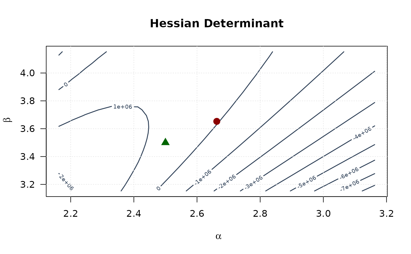
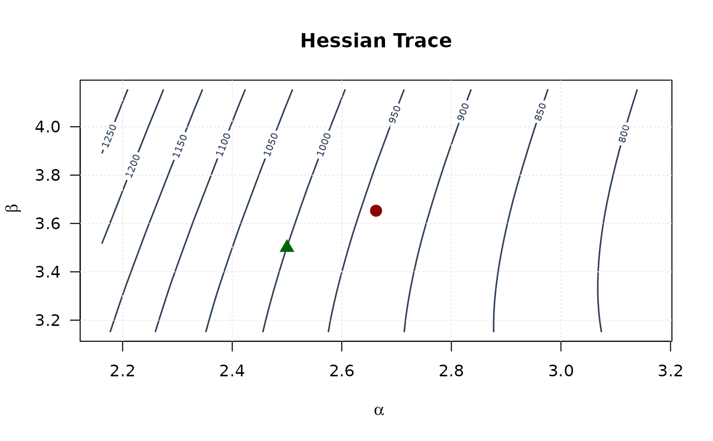
## Example 5: Curvature Visualization (Alpha vs Beta)
# Create grid around MLE
alpha_grid <- seq(mle[1] - 0.5, mle[1] + 0.5, length.out = 25)
beta_grid <- seq(mle[2] - 0.5, mle[2] + 0.5, length.out = 25)
alpha_grid <- alpha_grid[alpha_grid > 0]
beta_grid <- beta_grid[beta_grid > 0]
# Compute curvature measures
determinant_surface <- matrix(NA,
nrow = length(alpha_grid),
ncol = length(beta_grid)
)
trace_surface <- matrix(NA,
nrow = length(alpha_grid),
ncol = length(beta_grid)
)
for (i in seq_along(alpha_grid)) {
for (j in seq_along(beta_grid)) {
H <- hsekw(c(alpha_grid[i], beta_grid[j], mle[3]), data)
determinant_surface[i, j] <- det(H)
trace_surface[i, j] <- sum(diag(H))
}
}
# Plot
contour(alpha_grid, beta_grid, determinant_surface,
xlab = expression(alpha), ylab = expression(beta),
main = "Hessian Determinant", las = 1,
col = "#2E4057", lwd = 1.5, nlevels = 15
)
points(mle[1], mle[2], pch = 19, col = "#8B0000", cex = 1.5)
points(true_params[1], true_params[2], pch = 17, col = "#006400", cex = 1.5)
grid(col = "gray90")
 contour(alpha_grid, beta_grid, trace_surface,
xlab = expression(alpha), ylab = expression(beta),
main = "Hessian Trace", las = 1,
col = "#2E4057", lwd = 1.5, nlevels = 15
)
points(mle[1], mle[2], pch = 19, col = "#8B0000", cex = 1.5)
points(true_params[1], true_params[2], pch = 17, col = "#006400", cex = 1.5)
grid(col = "gray90")
contour(alpha_grid, beta_grid, trace_surface,
xlab = expression(alpha), ylab = expression(beta),
main = "Hessian Trace", las = 1,
col = "#2E4057", lwd = 1.5, nlevels = 15
)
points(mle[1], mle[2], pch = 19, col = "#8B0000", cex = 1.5)
points(true_params[1], true_params[2], pch = 17, col = "#006400", cex = 1.5)
grid(col = "gray90")
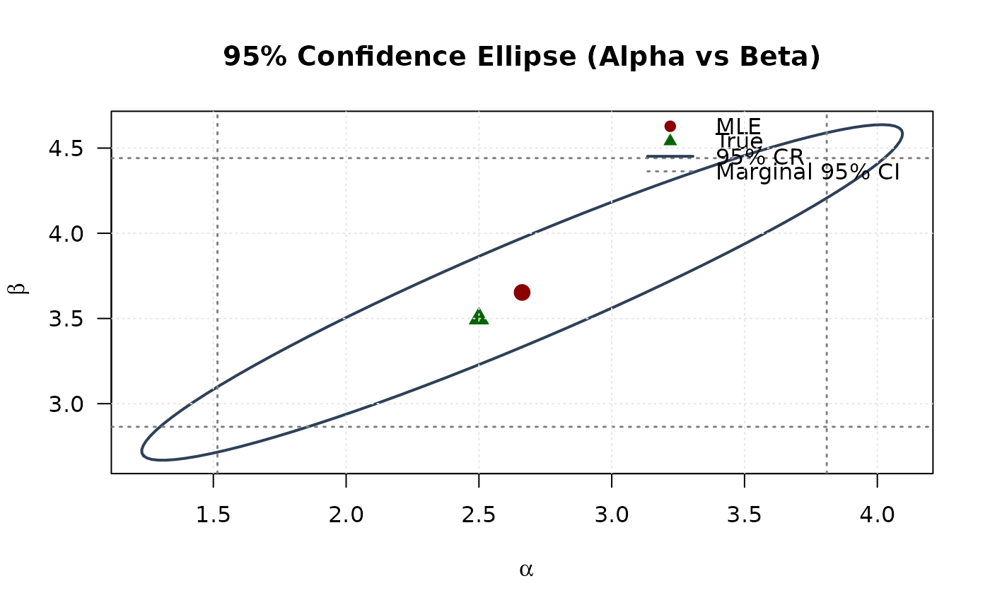
 ## Example 6: Confidence Ellipse (Alpha vs Beta)
# Extract 2x2 submatrix for alpha and beta
vcov_2d <- vcov_matrix[1:2, 1:2]
# Create confidence ellipse
theta <- seq(0, 2 * pi, length.out = 100)
chi2_val <- qchisq(0.95, df = 2)
eig_decomp <- eigen(vcov_2d)
ellipse <- matrix(NA, nrow = 100, ncol = 2)
for (i in 1:100) {
v <- c(cos(theta[i]), sin(theta[i]))
ellipse[i, ] <- mle[1:2] + sqrt(chi2_val) *
(eig_decomp$vectors %*% diag(sqrt(eig_decomp$values)) %*% v)
}
# Marginal confidence intervals
se_2d <- sqrt(diag(vcov_2d))
ci_alpha <- mle[1] + c(-1, 1) * 1.96 * se_2d[1]
ci_beta <- mle[2] + c(-1, 1) * 1.96 * se_2d[2]
# Plot
plot(ellipse[, 1], ellipse[, 2],
type = "l", lwd = 2, col = "#2E4057",
xlab = expression(alpha), ylab = expression(beta),
main = "95% Confidence Ellipse (Alpha vs Beta)", las = 1
)
# Add marginal CIs
abline(v = ci_alpha, col = "#808080", lty = 3, lwd = 1.5)
abline(h = ci_beta, col = "#808080", lty = 3, lwd = 1.5)
points(mle[1], mle[2], pch = 19, col = "#8B0000", cex = 1.5)
points(true_params[1], true_params[2], pch = 17, col = "#006400", cex = 1.5)
legend("topright",
legend = c("MLE", "True", "95% CR", "Marginal 95% CI"),
col = c("#8B0000", "#006400", "#2E4057", "#808080"),
pch = c(19, 17, NA, NA),
lty = c(NA, NA, 1, 3),
lwd = c(NA, NA, 2, 1.5),
bty = "n"
)
grid(col = "gray90")
## Example 6: Confidence Ellipse (Alpha vs Beta)
# Extract 2x2 submatrix for alpha and beta
vcov_2d <- vcov_matrix[1:2, 1:2]
# Create confidence ellipse
theta <- seq(0, 2 * pi, length.out = 100)
chi2_val <- qchisq(0.95, df = 2)
eig_decomp <- eigen(vcov_2d)
ellipse <- matrix(NA, nrow = 100, ncol = 2)
for (i in 1:100) {
v <- c(cos(theta[i]), sin(theta[i]))
ellipse[i, ] <- mle[1:2] + sqrt(chi2_val) *
(eig_decomp$vectors %*% diag(sqrt(eig_decomp$values)) %*% v)
}
# Marginal confidence intervals
se_2d <- sqrt(diag(vcov_2d))
ci_alpha <- mle[1] + c(-1, 1) * 1.96 * se_2d[1]
ci_beta <- mle[2] + c(-1, 1) * 1.96 * se_2d[2]
# Plot
plot(ellipse[, 1], ellipse[, 2],
type = "l", lwd = 2, col = "#2E4057",
xlab = expression(alpha), ylab = expression(beta),
main = "95% Confidence Ellipse (Alpha vs Beta)", las = 1
)
# Add marginal CIs
abline(v = ci_alpha, col = "#808080", lty = 3, lwd = 1.5)
abline(h = ci_beta, col = "#808080", lty = 3, lwd = 1.5)
points(mle[1], mle[2], pch = 19, col = "#8B0000", cex = 1.5)
points(true_params[1], true_params[2], pch = 17, col = "#006400", cex = 1.5)
legend("topright",
legend = c("MLE", "True", "95% CR", "Marginal 95% CI"),
col = c("#8B0000", "#006400", "#2E4057", "#808080"),
pch = c(19, 17, NA, NA),
lty = c(NA, NA, 1, 3),
lwd = c(NA, NA, 2, 1.5),
bty = "n"
)
grid(col = "gray90")
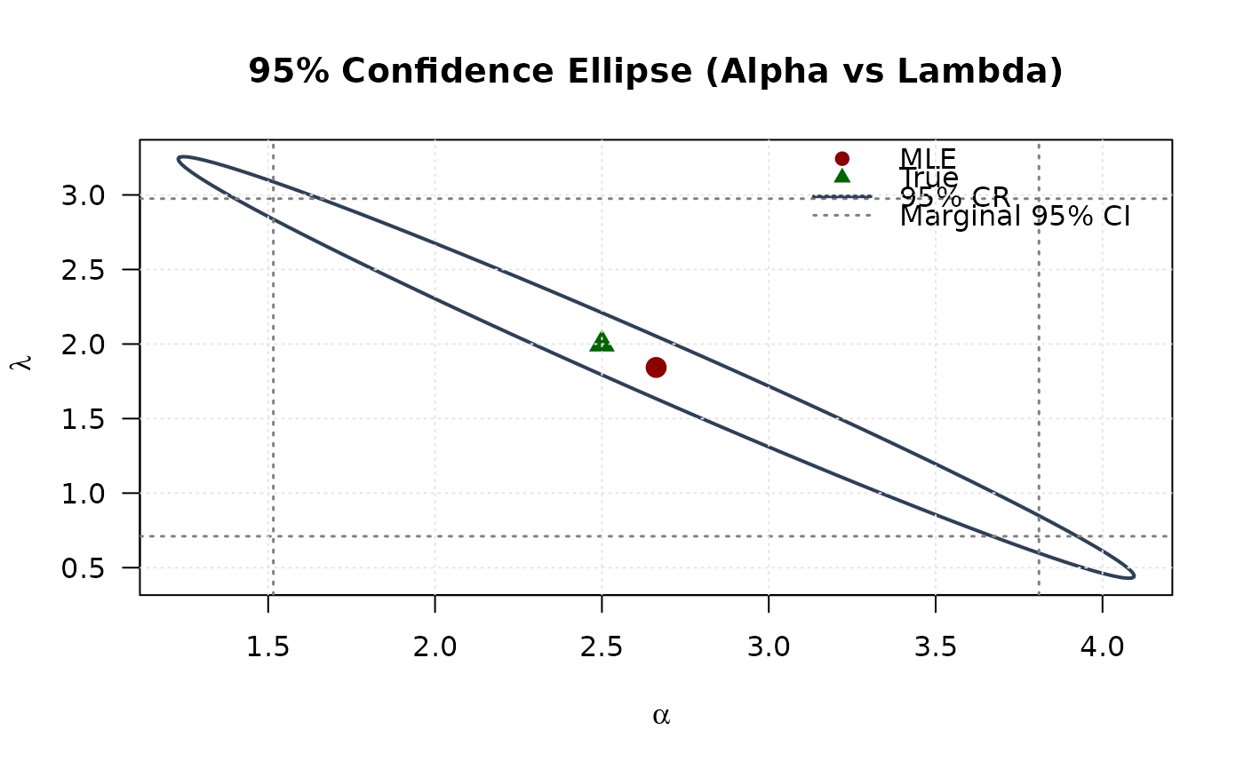
 ## Example 7: Confidence Ellipse (Alpha vs Lambda)
# Extract 2x2 submatrix for alpha and lambda
vcov_2d_al <- vcov_matrix[c(1, 3), c(1, 3)]
# Create confidence ellipse
eig_decomp_al <- eigen(vcov_2d_al)
ellipse_al <- matrix(NA, nrow = 100, ncol = 2)
for (i in 1:100) {
v <- c(cos(theta[i]), sin(theta[i]))
ellipse_al[i, ] <- mle[c(1, 3)] + sqrt(chi2_val) *
(eig_decomp_al$vectors %*% diag(sqrt(eig_decomp_al$values)) %*% v)
}
# Marginal confidence intervals
se_2d_al <- sqrt(diag(vcov_2d_al))
ci_alpha_2 <- mle[1] + c(-1, 1) * 1.96 * se_2d_al[1]
ci_lambda <- mle[3] + c(-1, 1) * 1.96 * se_2d_al[2]
# Plot
plot(ellipse_al[, 1], ellipse_al[, 2],
type = "l", lwd = 2, col = "#2E4057",
xlab = expression(alpha), ylab = expression(lambda),
main = "95% Confidence Ellipse (Alpha vs Lambda)", las = 1
)
# Add marginal CIs
abline(v = ci_alpha_2, col = "#808080", lty = 3, lwd = 1.5)
abline(h = ci_lambda, col = "#808080", lty = 3, lwd = 1.5)
points(mle[1], mle[3], pch = 19, col = "#8B0000", cex = 1.5)
points(true_params[1], true_params[3], pch = 17, col = "#006400", cex = 1.5)
legend("topright",
legend = c("MLE", "True", "95% CR", "Marginal 95% CI"),
col = c("#8B0000", "#006400", "#2E4057", "#808080"),
pch = c(19, 17, NA, NA),
lty = c(NA, NA, 1, 3),
lwd = c(NA, NA, 2, 1.5),
bty = "n"
)
grid(col = "gray90")
## Example 7: Confidence Ellipse (Alpha vs Lambda)
# Extract 2x2 submatrix for alpha and lambda
vcov_2d_al <- vcov_matrix[c(1, 3), c(1, 3)]
# Create confidence ellipse
eig_decomp_al <- eigen(vcov_2d_al)
ellipse_al <- matrix(NA, nrow = 100, ncol = 2)
for (i in 1:100) {
v <- c(cos(theta[i]), sin(theta[i]))
ellipse_al[i, ] <- mle[c(1, 3)] + sqrt(chi2_val) *
(eig_decomp_al$vectors %*% diag(sqrt(eig_decomp_al$values)) %*% v)
}
# Marginal confidence intervals
se_2d_al <- sqrt(diag(vcov_2d_al))
ci_alpha_2 <- mle[1] + c(-1, 1) * 1.96 * se_2d_al[1]
ci_lambda <- mle[3] + c(-1, 1) * 1.96 * se_2d_al[2]
# Plot
plot(ellipse_al[, 1], ellipse_al[, 2],
type = "l", lwd = 2, col = "#2E4057",
xlab = expression(alpha), ylab = expression(lambda),
main = "95% Confidence Ellipse (Alpha vs Lambda)", las = 1
)
# Add marginal CIs
abline(v = ci_alpha_2, col = "#808080", lty = 3, lwd = 1.5)
abline(h = ci_lambda, col = "#808080", lty = 3, lwd = 1.5)
points(mle[1], mle[3], pch = 19, col = "#8B0000", cex = 1.5)
points(true_params[1], true_params[3], pch = 17, col = "#006400", cex = 1.5)
legend("topright",
legend = c("MLE", "True", "95% CR", "Marginal 95% CI"),
col = c("#8B0000", "#006400", "#2E4057", "#808080"),
pch = c(19, 17, NA, NA),
lty = c(NA, NA, 1, 3),
lwd = c(NA, NA, 2, 1.5),
bty = "n"
)
grid(col = "gray90")
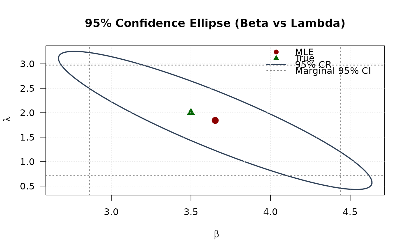
 ## Example 8: Confidence Ellipse (Beta vs Lambda)
# Extract 2x2 submatrix for beta and lambda
vcov_2d_bl <- vcov_matrix[2:3, 2:3]
# Create confidence ellipse
eig_decomp_bl <- eigen(vcov_2d_bl)
ellipse_bl <- matrix(NA, nrow = 100, ncol = 2)
for (i in 1:100) {
v <- c(cos(theta[i]), sin(theta[i]))
ellipse_bl[i, ] <- mle[2:3] + sqrt(chi2_val) *
(eig_decomp_bl$vectors %*% diag(sqrt(eig_decomp_bl$values)) %*% v)
}
# Marginal confidence intervals
se_2d_bl <- sqrt(diag(vcov_2d_bl))
ci_beta_2 <- mle[2] + c(-1, 1) * 1.96 * se_2d_bl[1]
ci_lambda_2 <- mle[3] + c(-1, 1) * 1.96 * se_2d_bl[2]
# Plot
plot(ellipse_bl[, 1], ellipse_bl[, 2],
type = "l", lwd = 2, col = "#2E4057",
xlab = expression(beta), ylab = expression(lambda),
main = "95% Confidence Ellipse (Beta vs Lambda)", las = 1
)
# Add marginal CIs
abline(v = ci_beta_2, col = "#808080", lty = 3, lwd = 1.5)
abline(h = ci_lambda_2, col = "#808080", lty = 3, lwd = 1.5)
points(mle[2], mle[3], pch = 19, col = "#8B0000", cex = 1.5)
points(true_params[2], true_params[3], pch = 17, col = "#006400", cex = 1.5)
legend("topright",
legend = c("MLE", "True", "95% CR", "Marginal 95% CI"),
col = c("#8B0000", "#006400", "#2E4057", "#808080"),
pch = c(19, 17, NA, NA),
lty = c(NA, NA, 1, 3),
lwd = c(NA, NA, 2, 1.5),
bty = "n"
)
grid(col = "gray90")
## Example 8: Confidence Ellipse (Beta vs Lambda)
# Extract 2x2 submatrix for beta and lambda
vcov_2d_bl <- vcov_matrix[2:3, 2:3]
# Create confidence ellipse
eig_decomp_bl <- eigen(vcov_2d_bl)
ellipse_bl <- matrix(NA, nrow = 100, ncol = 2)
for (i in 1:100) {
v <- c(cos(theta[i]), sin(theta[i]))
ellipse_bl[i, ] <- mle[2:3] + sqrt(chi2_val) *
(eig_decomp_bl$vectors %*% diag(sqrt(eig_decomp_bl$values)) %*% v)
}
# Marginal confidence intervals
se_2d_bl <- sqrt(diag(vcov_2d_bl))
ci_beta_2 <- mle[2] + c(-1, 1) * 1.96 * se_2d_bl[1]
ci_lambda_2 <- mle[3] + c(-1, 1) * 1.96 * se_2d_bl[2]
# Plot
plot(ellipse_bl[, 1], ellipse_bl[, 2],
type = "l", lwd = 2, col = "#2E4057",
xlab = expression(beta), ylab = expression(lambda),
main = "95% Confidence Ellipse (Beta vs Lambda)", las = 1
)
# Add marginal CIs
abline(v = ci_beta_2, col = "#808080", lty = 3, lwd = 1.5)
abline(h = ci_lambda_2, col = "#808080", lty = 3, lwd = 1.5)
points(mle[2], mle[3], pch = 19, col = "#8B0000", cex = 1.5)
points(true_params[2], true_params[3], pch = 17, col = "#006400", cex = 1.5)
legend("topright",
legend = c("MLE", "True", "95% CR", "Marginal 95% CI"),
col = c("#8B0000", "#006400", "#2E4057", "#808080"),
pch = c(19, 17, NA, NA),
lty = c(NA, NA, 1, 3),
lwd = c(NA, NA, 2, 1.5),
bty = "n"
)
grid(col = "gray90")
 # }
# }