Gradient of the Negative Log-Likelihood for the McDonald (Mc)/Beta Power Distribution
Source:R/bpmc.R
grmc.RdComputes the gradient vector (vector of first partial derivatives) of the
negative log-likelihood function for the McDonald (Mc) distribution (also
known as Beta Power) with parameters gamma (\(\gamma\)), delta
(\(\delta\)), and lambda (\(\lambda\)). This distribution is the
special case of the Generalized Kumaraswamy (GKw) distribution where
\(\alpha = 1\) and \(\beta = 1\). The gradient is useful for optimization.
Value
Returns a numeric vector of length 3 containing the partial derivatives
of the negative log-likelihood function \(-\ell(\theta | \mathbf{x})\) with
respect to each parameter:
\((-\partial \ell/\partial \gamma, -\partial \ell/\partial \delta, -\partial \ell/\partial \lambda)\).
Returns a vector of NaN if any parameter values are invalid according
to their constraints, or if any value in data is not in the
interval (0, 1).
Details
The components of the gradient vector of the negative log-likelihood (\(-\nabla \ell(\theta | \mathbf{x})\)) for the Mc (\(\alpha=1, \beta=1\)) model are:
$$ -\frac{\partial \ell}{\partial \gamma} = n[\psi(\gamma+\delta+1) - \psi(\gamma)] - \lambda\sum_{i=1}^{n}\ln(x_i) $$ $$ -\frac{\partial \ell}{\partial \delta} = n[\psi(\gamma+\delta+1) - \psi(\delta+1)] - \sum_{i=1}^{n}\ln(1-x_i^{\lambda}) $$ $$ -\frac{\partial \ell}{\partial \lambda} = -\frac{n}{\lambda} - \gamma\sum_{i=1}^{n}\ln(x_i) + \delta\sum_{i=1}^{n}\frac{x_i^{\lambda}\ln(x_i)}{1-x_i^{\lambda}} $$
where \(\psi(\cdot)\) is the digamma function (digamma).
These formulas represent the derivatives of \(-\ell(\theta)\), consistent with
minimizing the negative log-likelihood. They correspond to the relevant components
of the general GKw gradient (grgkw) evaluated at \(\alpha=1, \beta=1\).
References
McDonald, J. B. (1984). Some generalized functions for the size distribution of income. Econometrica, 52(3), 647-663.
Cordeiro, G. M., & de Castro, M. (2011). A new family of generalized distributions. Journal of Statistical Computation and Simulation,
(Note: Specific gradient formulas might be derived or sourced from additional references).
Examples
# \donttest{
## Example 1: Basic Examples
# Generate sample data with more stable parameters
set.seed(123)
n <- 1000
true_params <- c(gamma = 2.0, delta = 2.5, lambda = 1.5)
data <- rmc(n,
gamma = true_params[1], delta = true_params[2],
lambda = true_params[3]
)
# Evaluate Hessian at true parameters
hess_true <- hsmc(par = true_params, data = data)
cat("Hessian matrix at true parameters:\n")
#> Hessian matrix at true parameters:
print(hess_true, digits = 4)
#> [,1] [,2] [,3]
#> [1,] 445.6 -199.3 783.2
#> [2,] -199.3 131.0 -369.8
#> [3,] 783.2 -369.8 1416.2
# Check symmetry
cat(
"\nSymmetry check (max |H - H^T|):",
max(abs(hess_true - t(hess_true))), "\n"
)
#>
#> Symmetry check (max |H - H^T|): 0
## Example 2: Hessian Properties at MLE
# Fit model
fit <- optim(
par = c(1.5, 2.0, 1.0),
fn = llmc,
gr = grmc,
data = data,
method = "BFGS",
hessian = TRUE
)
mle <- fit$par
names(mle) <- c("gamma", "delta", "lambda")
# Hessian at MLE
hessian_at_mle <- hsmc(par = mle, data = data)
cat("\nHessian at MLE:\n")
#>
#> Hessian at MLE:
print(hessian_at_mle, digits = 4)
#> [,1] [,2] [,3]
#> [1,] 754.3 -216.43 783.2
#> [2,] -216.4 99.01 -238.6
#> [3,] 783.2 -238.57 820.1
# Compare with optim's numerical Hessian
cat("\nComparison with optim Hessian:\n")
#>
#> Comparison with optim Hessian:
cat(
"Max absolute difference:",
max(abs(hessian_at_mle - fit$hessian)), "\n"
)
#> Max absolute difference: 0.0002574138
# Eigenvalue analysis
eigenvals <- eigen(hessian_at_mle, only.values = TRUE)$values
cat("\nEigenvalues:\n")
#>
#> Eigenvalues:
print(eigenvals)
#> [1] 1638.4186859 34.1207859 0.8213602
cat("\nPositive definite:", all(eigenvals > 0), "\n")
#>
#> Positive definite: TRUE
cat("Condition number:", max(eigenvals) / min(eigenvals), "\n")
#> Condition number: 1994.763
## Example 3: Standard Errors and Confidence Intervals
# Observed information matrix
obs_info <- hessian_at_mle
# Variance-covariance matrix
vcov_matrix <- solve(obs_info)
cat("\nVariance-Covariance Matrix:\n")
#>
#> Variance-Covariance Matrix:
print(vcov_matrix, digits = 6)
#> [,1] [,2] [,3]
#> [1,] 0.528826 -0.203770 -0.564330
#> [2,] -0.203770 0.112290 0.227275
#> [3,] -0.564330 0.227275 0.606294
# Standard errors
se <- sqrt(diag(vcov_matrix))
names(se) <- c("gamma", "delta", "lambda")
# Correlation matrix
corr_matrix <- cov2cor(vcov_matrix)
cat("\nCorrelation Matrix:\n")
#>
#> Correlation Matrix:
print(corr_matrix, digits = 4)
#> [,1] [,2] [,3]
#> [1,] 1.0000 -0.8362 -0.9966
#> [2,] -0.8362 1.0000 0.8710
#> [3,] -0.9966 0.8710 1.0000
# Confidence intervals
z_crit <- qnorm(0.975)
results <- data.frame(
Parameter = c("gamma", "delta", "lambda"),
True = true_params,
MLE = mle,
SE = se,
CI_Lower = mle - z_crit * se,
CI_Upper = mle + z_crit * se
)
print(results, digits = 4)
#> Parameter True MLE SE CI_Lower CI_Upper
#> gamma gamma 2.0 1.458 0.7272 0.03292 2.884
#> delta delta 2.5 2.644 0.3351 1.98755 3.301
#> lambda lambda 1.5 1.956 0.7786 0.42971 3.482
## Example 4: Determinant and Trace Analysis
# Compute at different points
test_params <- rbind(
c(1.5, 2.0, 1.0),
c(2.0, 2.5, 1.5),
mle,
c(2.5, 3.0, 2.0)
)
hess_properties <- data.frame(
Gamma = numeric(),
Delta = numeric(),
Lambda = numeric(),
Determinant = numeric(),
Trace = numeric(),
Min_Eigenval = numeric(),
Max_Eigenval = numeric(),
Cond_Number = numeric(),
stringsAsFactors = FALSE
)
for (i in 1:nrow(test_params)) {
H <- hsmc(par = test_params[i, ], data = data)
eigs <- eigen(H, only.values = TRUE)$values
hess_properties <- rbind(hess_properties, data.frame(
Gamma = test_params[i, 1],
Delta = test_params[i, 2],
Lambda = test_params[i, 3],
Determinant = det(H),
Trace = sum(diag(H)),
Min_Eigenval = min(eigs),
Max_Eigenval = max(eigs),
Cond_Number = max(eigs) / min(eigs)
))
}
cat("\nHessian Properties at Different Points:\n")
#>
#> Hessian Properties at Different Points:
print(hess_properties, digits = 4, row.names = FALSE)
#> Gamma Delta Lambda Determinant Trace Min_Eigenval Max_Eigenval Cond_Number
#> 1.500 2.000 1.000 -28036436 3709 -19.4941 3292 -168.864
#> 2.000 2.500 1.500 569493 1993 8.3039 1949 234.745
#> 1.458 2.644 1.956 45917 1673 0.8214 1638 1994.763
#> 2.500 3.000 2.000 -20506346 1293 -238.7457 1473 -6.171
## Example 5: Curvature Visualization (All pairs side by side)
# Create grids around MLE with wider range (±1.5)
gamma_grid <- seq(mle[1] - 1.5, mle[1] + 1.5, length.out = 25)
delta_grid <- seq(mle[2] - 1.5, mle[2] + 1.5, length.out = 25)
lambda_grid <- seq(mle[3] - 1.5, mle[3] + 1.5, length.out = 25)
gamma_grid <- gamma_grid[gamma_grid > 0]
delta_grid <- delta_grid[delta_grid > 0]
lambda_grid <- lambda_grid[lambda_grid > 0]
# Compute curvature measures for all pairs
determinant_surface_gd <- matrix(NA, nrow = length(gamma_grid), ncol = length(delta_grid))
trace_surface_gd <- matrix(NA, nrow = length(gamma_grid), ncol = length(delta_grid))
determinant_surface_gl <- matrix(NA, nrow = length(gamma_grid), ncol = length(lambda_grid))
trace_surface_gl <- matrix(NA, nrow = length(gamma_grid), ncol = length(lambda_grid))
determinant_surface_dl <- matrix(NA, nrow = length(delta_grid), ncol = length(lambda_grid))
trace_surface_dl <- matrix(NA, nrow = length(delta_grid), ncol = length(lambda_grid))
# Gamma vs Delta
for (i in seq_along(gamma_grid)) {
for (j in seq_along(delta_grid)) {
H <- hsmc(c(gamma_grid[i], delta_grid[j], mle[3]), data)
determinant_surface_gd[i, j] <- det(H)
trace_surface_gd[i, j] <- sum(diag(H))
}
}
# Gamma vs Lambda
for (i in seq_along(gamma_grid)) {
for (j in seq_along(lambda_grid)) {
H <- hsmc(c(gamma_grid[i], mle[2], lambda_grid[j]), data)
determinant_surface_gl[i, j] <- det(H)
trace_surface_gl[i, j] <- sum(diag(H))
}
}
# Delta vs Lambda
for (i in seq_along(delta_grid)) {
for (j in seq_along(lambda_grid)) {
H <- hsmc(c(mle[1], delta_grid[i], lambda_grid[j]), data)
determinant_surface_dl[i, j] <- det(H)
trace_surface_dl[i, j] <- sum(diag(H))
}
}
# Plot
# Determinant plots
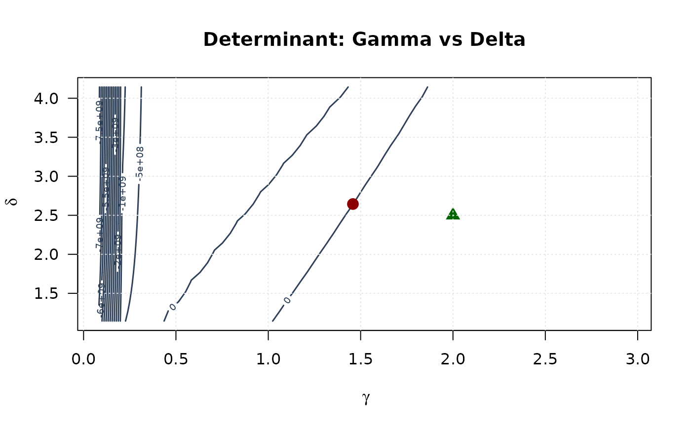
contour(gamma_grid, delta_grid, determinant_surface_gd,
xlab = expression(gamma), ylab = expression(delta),
main = "Determinant: Gamma vs Delta", las = 1,
col = "#2E4057", lwd = 1.5, nlevels = 15
)
points(mle[1], mle[2], pch = 19, col = "#8B0000", cex = 1.5)
points(true_params[1], true_params[2], pch = 17, col = "#006400", cex = 1.5)
grid(col = "gray90")
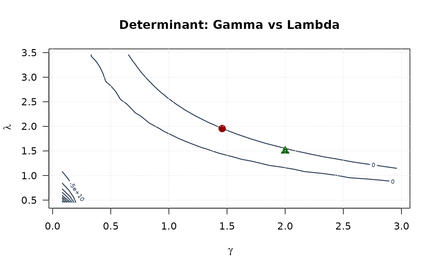
 contour(gamma_grid, lambda_grid, determinant_surface_gl,
xlab = expression(gamma), ylab = expression(lambda),
main = "Determinant: Gamma vs Lambda", las = 1,
col = "#2E4057", lwd = 1.5, nlevels = 15
)
points(mle[1], mle[3], pch = 19, col = "#8B0000", cex = 1.5)
points(true_params[1], true_params[3], pch = 17, col = "#006400", cex = 1.5)
grid(col = "gray90")
contour(gamma_grid, lambda_grid, determinant_surface_gl,
xlab = expression(gamma), ylab = expression(lambda),
main = "Determinant: Gamma vs Lambda", las = 1,
col = "#2E4057", lwd = 1.5, nlevels = 15
)
points(mle[1], mle[3], pch = 19, col = "#8B0000", cex = 1.5)
points(true_params[1], true_params[3], pch = 17, col = "#006400", cex = 1.5)
grid(col = "gray90")
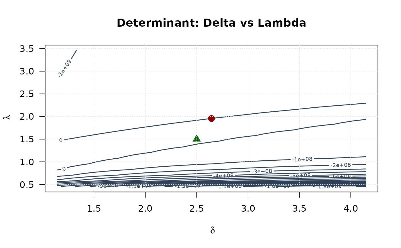
 contour(delta_grid, lambda_grid, determinant_surface_dl,
xlab = expression(delta), ylab = expression(lambda),
main = "Determinant: Delta vs Lambda", las = 1,
col = "#2E4057", lwd = 1.5, nlevels = 15
)
points(mle[2], mle[3], pch = 19, col = "#8B0000", cex = 1.5)
points(true_params[2], true_params[3], pch = 17, col = "#006400", cex = 1.5)
grid(col = "gray90")
contour(delta_grid, lambda_grid, determinant_surface_dl,
xlab = expression(delta), ylab = expression(lambda),
main = "Determinant: Delta vs Lambda", las = 1,
col = "#2E4057", lwd = 1.5, nlevels = 15
)
points(mle[2], mle[3], pch = 19, col = "#8B0000", cex = 1.5)
points(true_params[2], true_params[3], pch = 17, col = "#006400", cex = 1.5)
grid(col = "gray90")
 # Trace plots
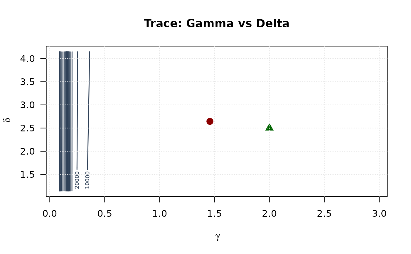
contour(gamma_grid, delta_grid, trace_surface_gd,
xlab = expression(gamma), ylab = expression(delta),
main = "Trace: Gamma vs Delta", las = 1,
col = "#2E4057", lwd = 1.5, nlevels = 15
)
points(mle[1], mle[2], pch = 19, col = "#8B0000", cex = 1.5)
points(true_params[1], true_params[2], pch = 17, col = "#006400", cex = 1.5)
grid(col = "gray90")
# Trace plots
contour(gamma_grid, delta_grid, trace_surface_gd,
xlab = expression(gamma), ylab = expression(delta),
main = "Trace: Gamma vs Delta", las = 1,
col = "#2E4057", lwd = 1.5, nlevels = 15
)
points(mle[1], mle[2], pch = 19, col = "#8B0000", cex = 1.5)
points(true_params[1], true_params[2], pch = 17, col = "#006400", cex = 1.5)
grid(col = "gray90")
 contour(gamma_grid, lambda_grid, trace_surface_gl,
xlab = expression(gamma), ylab = expression(lambda),
main = "Trace: Gamma vs Lambda", las = 1,
col = "#2E4057", lwd = 1.5, nlevels = 15
)
points(mle[1], mle[3], pch = 19, col = "#8B0000", cex = 1.5)
points(true_params[1], true_params[3], pch = 17, col = "#006400", cex = 1.5)
grid(col = "gray90")
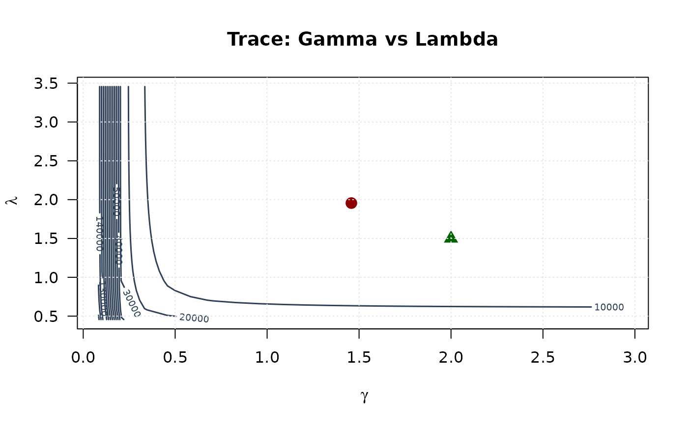
contour(gamma_grid, lambda_grid, trace_surface_gl,
xlab = expression(gamma), ylab = expression(lambda),
main = "Trace: Gamma vs Lambda", las = 1,
col = "#2E4057", lwd = 1.5, nlevels = 15
)
points(mle[1], mle[3], pch = 19, col = "#8B0000", cex = 1.5)
points(true_params[1], true_params[3], pch = 17, col = "#006400", cex = 1.5)
grid(col = "gray90")
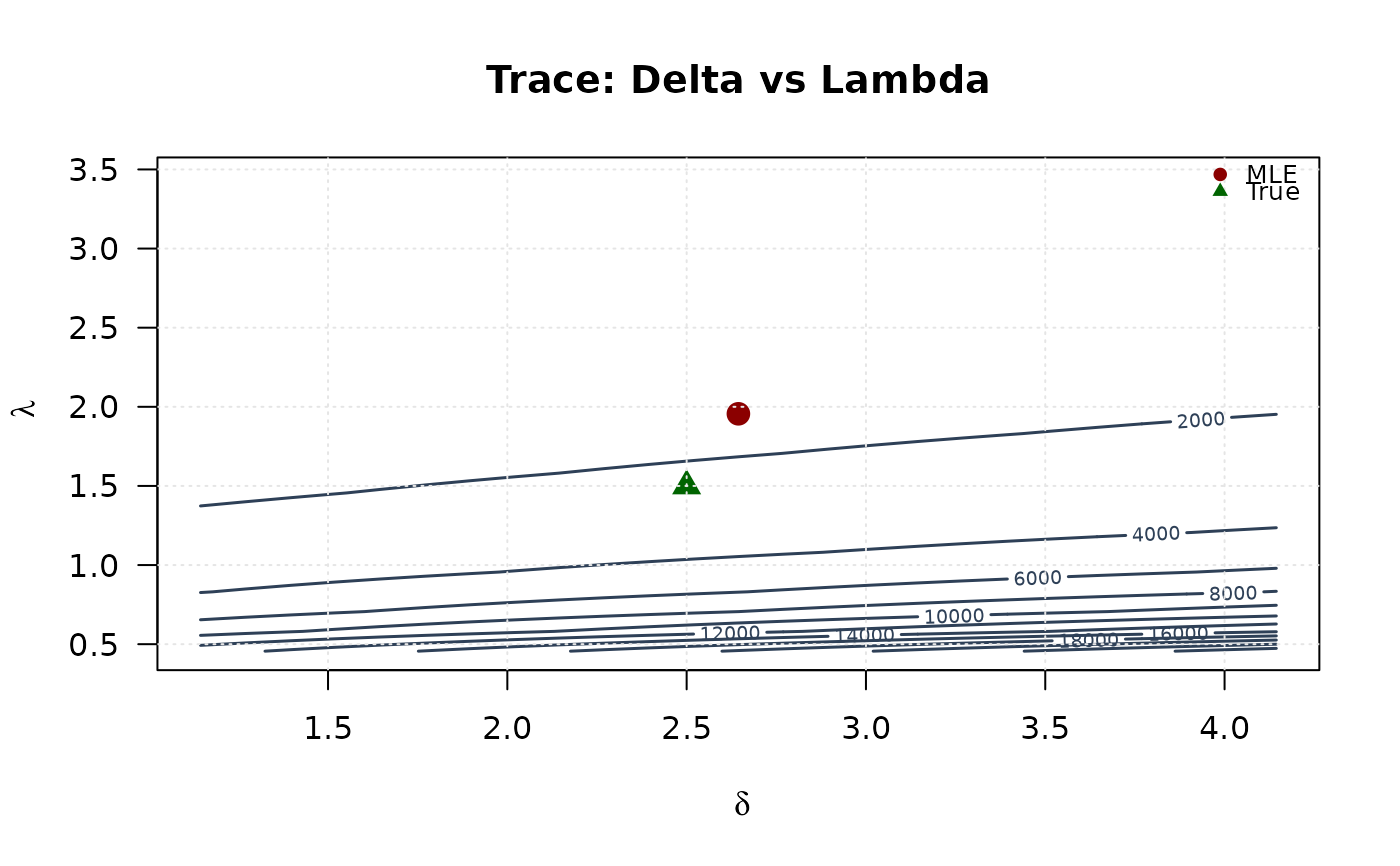
 contour(delta_grid, lambda_grid, trace_surface_dl,
xlab = expression(delta), ylab = expression(lambda),
main = "Trace: Delta vs Lambda", las = 1,
col = "#2E4057", lwd = 1.5, nlevels = 15
)
points(mle[2], mle[3], pch = 19, col = "#8B0000", cex = 1.5)
points(true_params[2], true_params[3], pch = 17, col = "#006400", cex = 1.5)
grid(col = "gray90")
legend("topright",
legend = c("MLE", "True"),
col = c("#8B0000", "#006400"),
pch = c(19, 17),
bty = "n", cex = 0.8
)
contour(delta_grid, lambda_grid, trace_surface_dl,
xlab = expression(delta), ylab = expression(lambda),
main = "Trace: Delta vs Lambda", las = 1,
col = "#2E4057", lwd = 1.5, nlevels = 15
)
points(mle[2], mle[3], pch = 19, col = "#8B0000", cex = 1.5)
points(true_params[2], true_params[3], pch = 17, col = "#006400", cex = 1.5)
grid(col = "gray90")
legend("topright",
legend = c("MLE", "True"),
col = c("#8B0000", "#006400"),
pch = c(19, 17),
bty = "n", cex = 0.8
)
 ## Example 6: Confidence Ellipses (All pairs side by side)
# Extract all 2x2 submatrices
vcov_gd <- vcov_matrix[1:2, 1:2]
vcov_gl <- vcov_matrix[c(1, 3), c(1, 3)]
vcov_dl <- vcov_matrix[2:3, 2:3]
# Create confidence ellipses
theta <- seq(0, 2 * pi, length.out = 100)
chi2_val <- qchisq(0.95, df = 2)
# Gamma vs Delta ellipse
eig_decomp_gd <- eigen(vcov_gd)
ellipse_gd <- matrix(NA, nrow = 100, ncol = 2)
for (i in 1:100) {
v <- c(cos(theta[i]), sin(theta[i]))
ellipse_gd[i, ] <- mle[1:2] + sqrt(chi2_val) *
(eig_decomp_gd$vectors %*% diag(sqrt(eig_decomp_gd$values)) %*% v)
}
# Gamma vs Lambda ellipse
eig_decomp_gl <- eigen(vcov_gl)
ellipse_gl <- matrix(NA, nrow = 100, ncol = 2)
for (i in 1:100) {
v <- c(cos(theta[i]), sin(theta[i]))
ellipse_gl[i, ] <- mle[c(1, 3)] + sqrt(chi2_val) *
(eig_decomp_gl$vectors %*% diag(sqrt(eig_decomp_gl$values)) %*% v)
}
# Delta vs Lambda ellipse
eig_decomp_dl <- eigen(vcov_dl)
ellipse_dl <- matrix(NA, nrow = 100, ncol = 2)
for (i in 1:100) {
v <- c(cos(theta[i]), sin(theta[i]))
ellipse_dl[i, ] <- mle[2:3] + sqrt(chi2_val) *
(eig_decomp_dl$vectors %*% diag(sqrt(eig_decomp_dl$values)) %*% v)
}
# Marginal confidence intervals
se_gd <- sqrt(diag(vcov_gd))
ci_gamma_gd <- mle[1] + c(-1, 1) * 1.96 * se_gd[1]
ci_delta_gd <- mle[2] + c(-1, 1) * 1.96 * se_gd[2]
se_gl <- sqrt(diag(vcov_gl))
ci_gamma_gl <- mle[1] + c(-1, 1) * 1.96 * se_gl[1]
ci_lambda_gl <- mle[3] + c(-1, 1) * 1.96 * se_gl[2]
se_dl <- sqrt(diag(vcov_dl))
ci_delta_dl <- mle[2] + c(-1, 1) * 1.96 * se_dl[1]
ci_lambda_dl <- mle[3] + c(-1, 1) * 1.96 * se_dl[2]
# Plot
# Gamma vs Delta
plot(ellipse_gd[, 1], ellipse_gd[, 2],
type = "l", lwd = 2, col = "#2E4057",
xlab = expression(gamma), ylab = expression(delta),
main = "Gamma vs Delta", las = 1, xlim = range(ellipse_gd[, 1], ci_gamma_gd),
ylim = range(ellipse_gd[, 2], ci_delta_gd)
)
abline(v = ci_gamma_gd, col = "#808080", lty = 3, lwd = 1.5)
abline(h = ci_delta_gd, col = "#808080", lty = 3, lwd = 1.5)
points(mle[1], mle[2], pch = 19, col = "#8B0000", cex = 1.5)
points(true_params[1], true_params[2], pch = 17, col = "#006400", cex = 1.5)
grid(col = "gray90")
## Example 6: Confidence Ellipses (All pairs side by side)
# Extract all 2x2 submatrices
vcov_gd <- vcov_matrix[1:2, 1:2]
vcov_gl <- vcov_matrix[c(1, 3), c(1, 3)]
vcov_dl <- vcov_matrix[2:3, 2:3]
# Create confidence ellipses
theta <- seq(0, 2 * pi, length.out = 100)
chi2_val <- qchisq(0.95, df = 2)
# Gamma vs Delta ellipse
eig_decomp_gd <- eigen(vcov_gd)
ellipse_gd <- matrix(NA, nrow = 100, ncol = 2)
for (i in 1:100) {
v <- c(cos(theta[i]), sin(theta[i]))
ellipse_gd[i, ] <- mle[1:2] + sqrt(chi2_val) *
(eig_decomp_gd$vectors %*% diag(sqrt(eig_decomp_gd$values)) %*% v)
}
# Gamma vs Lambda ellipse
eig_decomp_gl <- eigen(vcov_gl)
ellipse_gl <- matrix(NA, nrow = 100, ncol = 2)
for (i in 1:100) {
v <- c(cos(theta[i]), sin(theta[i]))
ellipse_gl[i, ] <- mle[c(1, 3)] + sqrt(chi2_val) *
(eig_decomp_gl$vectors %*% diag(sqrt(eig_decomp_gl$values)) %*% v)
}
# Delta vs Lambda ellipse
eig_decomp_dl <- eigen(vcov_dl)
ellipse_dl <- matrix(NA, nrow = 100, ncol = 2)
for (i in 1:100) {
v <- c(cos(theta[i]), sin(theta[i]))
ellipse_dl[i, ] <- mle[2:3] + sqrt(chi2_val) *
(eig_decomp_dl$vectors %*% diag(sqrt(eig_decomp_dl$values)) %*% v)
}
# Marginal confidence intervals
se_gd <- sqrt(diag(vcov_gd))
ci_gamma_gd <- mle[1] + c(-1, 1) * 1.96 * se_gd[1]
ci_delta_gd <- mle[2] + c(-1, 1) * 1.96 * se_gd[2]
se_gl <- sqrt(diag(vcov_gl))
ci_gamma_gl <- mle[1] + c(-1, 1) * 1.96 * se_gl[1]
ci_lambda_gl <- mle[3] + c(-1, 1) * 1.96 * se_gl[2]
se_dl <- sqrt(diag(vcov_dl))
ci_delta_dl <- mle[2] + c(-1, 1) * 1.96 * se_dl[1]
ci_lambda_dl <- mle[3] + c(-1, 1) * 1.96 * se_dl[2]
# Plot
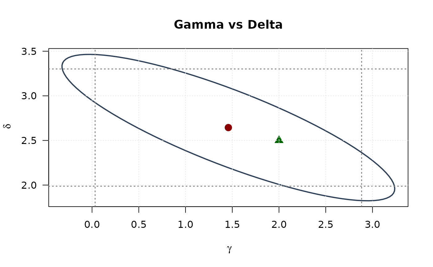
# Gamma vs Delta
plot(ellipse_gd[, 1], ellipse_gd[, 2],
type = "l", lwd = 2, col = "#2E4057",
xlab = expression(gamma), ylab = expression(delta),
main = "Gamma vs Delta", las = 1, xlim = range(ellipse_gd[, 1], ci_gamma_gd),
ylim = range(ellipse_gd[, 2], ci_delta_gd)
)
abline(v = ci_gamma_gd, col = "#808080", lty = 3, lwd = 1.5)
abline(h = ci_delta_gd, col = "#808080", lty = 3, lwd = 1.5)
points(mle[1], mle[2], pch = 19, col = "#8B0000", cex = 1.5)
points(true_params[1], true_params[2], pch = 17, col = "#006400", cex = 1.5)
grid(col = "gray90")
 # Gamma vs Lambda
plot(ellipse_gl[, 1], ellipse_gl[, 2],
type = "l", lwd = 2, col = "#2E4057",
xlab = expression(gamma), ylab = expression(lambda),
main = "Gamma vs Lambda", las = 1, xlim = range(ellipse_gl[, 1], ci_gamma_gl),
ylim = range(ellipse_gl[, 2], ci_lambda_gl)
)
abline(v = ci_gamma_gl, col = "#808080", lty = 3, lwd = 1.5)
abline(h = ci_lambda_gl, col = "#808080", lty = 3, lwd = 1.5)
points(mle[1], mle[3], pch = 19, col = "#8B0000", cex = 1.5)
points(true_params[1], true_params[3], pch = 17, col = "#006400", cex = 1.5)
grid(col = "gray90")
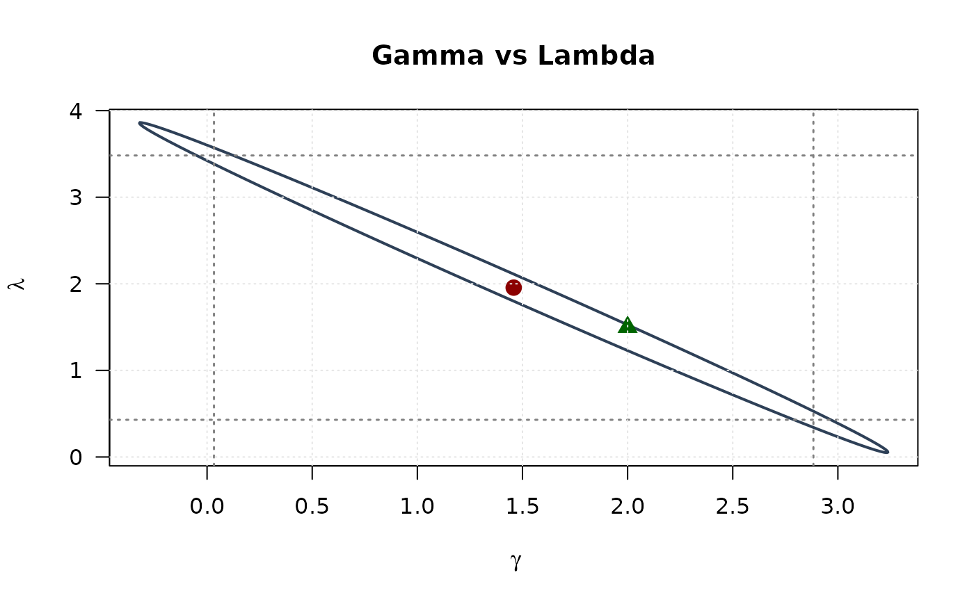
# Gamma vs Lambda
plot(ellipse_gl[, 1], ellipse_gl[, 2],
type = "l", lwd = 2, col = "#2E4057",
xlab = expression(gamma), ylab = expression(lambda),
main = "Gamma vs Lambda", las = 1, xlim = range(ellipse_gl[, 1], ci_gamma_gl),
ylim = range(ellipse_gl[, 2], ci_lambda_gl)
)
abline(v = ci_gamma_gl, col = "#808080", lty = 3, lwd = 1.5)
abline(h = ci_lambda_gl, col = "#808080", lty = 3, lwd = 1.5)
points(mle[1], mle[3], pch = 19, col = "#8B0000", cex = 1.5)
points(true_params[1], true_params[3], pch = 17, col = "#006400", cex = 1.5)
grid(col = "gray90")
 # Delta vs Lambda
plot(ellipse_dl[, 1], ellipse_dl[, 2],
type = "l", lwd = 2, col = "#2E4057",
xlab = expression(delta), ylab = expression(lambda),
main = "Delta vs Lambda", las = 1, xlim = range(ellipse_dl[, 1], ci_delta_dl),
ylim = range(ellipse_dl[, 2], ci_lambda_dl)
)
abline(v = ci_delta_dl, col = "#808080", lty = 3, lwd = 1.5)
abline(h = ci_lambda_dl, col = "#808080", lty = 3, lwd = 1.5)
points(mle[2], mle[3], pch = 19, col = "#8B0000", cex = 1.5)
points(true_params[2], true_params[3], pch = 17, col = "#006400", cex = 1.5)
grid(col = "gray90")
legend("topright",
legend = c("MLE", "True", "95% CR", "Marginal 95% CI"),
col = c("#8B0000", "#006400", "#2E4057", "#808080"),
pch = c(19, 17, NA, NA),
lty = c(NA, NA, 1, 3),
lwd = c(NA, NA, 2, 1.5),
bty = "n", cex = 0.8
)
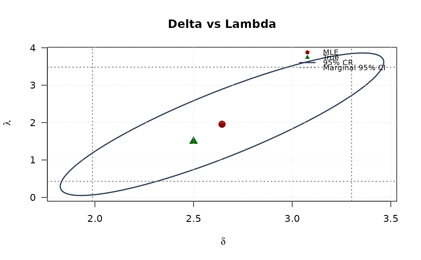
# Delta vs Lambda
plot(ellipse_dl[, 1], ellipse_dl[, 2],
type = "l", lwd = 2, col = "#2E4057",
xlab = expression(delta), ylab = expression(lambda),
main = "Delta vs Lambda", las = 1, xlim = range(ellipse_dl[, 1], ci_delta_dl),
ylim = range(ellipse_dl[, 2], ci_lambda_dl)
)
abline(v = ci_delta_dl, col = "#808080", lty = 3, lwd = 1.5)
abline(h = ci_lambda_dl, col = "#808080", lty = 3, lwd = 1.5)
points(mle[2], mle[3], pch = 19, col = "#8B0000", cex = 1.5)
points(true_params[2], true_params[3], pch = 17, col = "#006400", cex = 1.5)
grid(col = "gray90")
legend("topright",
legend = c("MLE", "True", "95% CR", "Marginal 95% CI"),
col = c("#8B0000", "#006400", "#2E4057", "#808080"),
pch = c(19, 17, NA, NA),
lty = c(NA, NA, 1, 3),
lwd = c(NA, NA, 2, 1.5),
bty = "n", cex = 0.8
)
 # }
# }