Gradient of the Negative Log-Likelihood for the Kumaraswamy (Kw) Distribution
Source:R/kw.R
grkw.RdComputes the gradient vector (vector of first partial derivatives) of the
negative log-likelihood function for the two-parameter Kumaraswamy (Kw)
distribution with parameters alpha (\(\alpha\)) and beta
(\(\beta\)). This provides the analytical gradient often used for efficient
optimization via maximum likelihood estimation.
Value
Returns a numeric vector of length 2 containing the partial derivatives
of the negative log-likelihood function \(-\ell(\theta | \mathbf{x})\) with
respect to each parameter: \((-\partial \ell/\partial \alpha, -\partial \ell/\partial \beta)\).
Returns a vector of NaN if any parameter values are invalid according
to their constraints, or if any value in data is not in the
interval (0, 1).
Details
The components of the gradient vector of the negative log-likelihood (\(-\nabla \ell(\theta | \mathbf{x})\)) for the Kw model are:
$$ -\frac{\partial \ell}{\partial \alpha} = -\frac{n}{\alpha} - \sum_{i=1}^{n}\ln(x_i) + (\beta-1)\sum_{i=1}^{n}\frac{x_i^{\alpha}\ln(x_i)}{v_i} $$ $$ -\frac{\partial \ell}{\partial \beta} = -\frac{n}{\beta} - \sum_{i=1}^{n}\ln(v_i) $$
where \(v_i = 1 - x_i^{\alpha}\).
These formulas represent the derivatives of \(-\ell(\theta)\), consistent with
minimizing the negative log-likelihood. They correspond to the relevant components
of the general GKw gradient (grgkw) evaluated at \(\gamma=1, \delta=0, \lambda=1\).
References
Kumaraswamy, P. (1980). A generalized probability density function for double-bounded random processes. Journal of Hydrology, 46(1-2), 79-88.
Jones, M. C. (2009). Kumaraswamy's distribution: A beta-type distribution with some tractability advantages. Statistical Methodology, 6(1), 70-81.
(Note: Specific gradient formulas might be derived or sourced from additional references).
Examples
# \donttest{
## Example 1: Basic Gradient Evaluation
# Generate sample data
set.seed(123)
n <- 1000
true_params <- c(alpha = 2.5, beta = 3.5)
data <- rkw(n, alpha = true_params[1], beta = true_params[2])
# Evaluate gradient at true parameters
grad_true <- grkw(par = true_params, data = data)
cat("Gradient at true parameters:\n")
#> Gradient at true parameters:
print(grad_true)
#> [1] 5.795703 -3.955898
cat("Norm:", sqrt(sum(grad_true^2)), "\n")
#> Norm: 7.017072
# Evaluate at different parameter values
test_params <- rbind(
c(1.5, 2.5),
c(2.0, 3.0),
c(2.5, 3.5),
c(3.0, 4.0)
)
grad_norms <- apply(test_params, 1, function(p) {
g <- grkw(p, data)
sqrt(sum(g^2))
})
results <- data.frame(
Alpha = test_params[, 1],
Beta = test_params[, 2],
Grad_Norm = grad_norms
)
print(results, digits = 4)
#> Alpha Beta Grad_Norm
#> 1 1.5 2.5 448.520
#> 2 2.0 3.0 175.451
#> 3 2.5 3.5 7.017
#> 4 3.0 4.0 137.615
## Example 2: Gradient in Optimization
# Optimization with analytical gradient
fit_with_grad <- optim(
par = c(2, 2),
fn = llkw,
gr = grkw,
data = data,
method = "BFGS",
hessian = TRUE,
control = list(trace = 0)
)
# Optimization without gradient
fit_no_grad <- optim(
par = c(2, 2),
fn = llkw,
data = data,
method = "BFGS",
hessian = TRUE,
control = list(trace = 0)
)
comparison <- data.frame(
Method = c("With Gradient", "Without Gradient"),
Alpha = c(fit_with_grad$par[1], fit_no_grad$par[1]),
Beta = c(fit_with_grad$par[2], fit_no_grad$par[2]),
NegLogLik = c(fit_with_grad$value, fit_no_grad$value),
Iterations = c(fit_with_grad$counts[1], fit_no_grad$counts[1])
)
print(comparison, digits = 4, row.names = FALSE)
#> Method Alpha Beta NegLogLik Iterations
#> With Gradient 2.511 3.571 -279.6 30
#> Without Gradient 2.511 3.571 -279.6 31
## Example 3: Verifying Gradient at MLE
mle <- fit_with_grad$par
names(mle) <- c("alpha", "beta")
# At MLE, gradient should be approximately zero
gradient_at_mle <- grkw(par = mle, data = data)
cat("\nGradient at MLE:\n")
#>
#> Gradient at MLE:
print(gradient_at_mle)
#> [1] 2.071782e-05 -1.146518e-05
cat("Max absolute component:", max(abs(gradient_at_mle)), "\n")
#> Max absolute component: 2.071782e-05
cat("Gradient norm:", sqrt(sum(gradient_at_mle^2)), "\n")
#> Gradient norm: 2.367865e-05
## Example 4: Numerical vs Analytical Gradient
# Manual finite difference gradient
numerical_gradient <- function(f, x, data, h = 1e-7) {
grad <- numeric(length(x))
for (i in seq_along(x)) {
x_plus <- x_minus <- x
x_plus[i] <- x[i] + h
x_minus[i] <- x[i] - h
grad[i] <- (f(x_plus, data) - f(x_minus, data)) / (2 * h)
}
return(grad)
}
# Compare at several points
test_points <- rbind(
c(1.5, 2.5),
c(2.0, 3.0),
mle,
c(3.0, 4.0)
)
cat("\nNumerical vs Analytical Gradient Comparison:\n")
#>
#> Numerical vs Analytical Gradient Comparison:
for (i in 1:nrow(test_points)) {
grad_analytical <- grkw(par = test_points[i, ], data = data)
grad_numerical <- numerical_gradient(llkw, test_points[i, ], data)
cat(
"\nPoint", i, ": alpha =", test_points[i, 1],
", beta =", test_points[i, 2], "\n"
)
comparison <- data.frame(
Parameter = c("alpha", "beta"),
Analytical = grad_analytical,
Numerical = grad_numerical,
Abs_Diff = abs(grad_analytical - grad_numerical),
Rel_Error = abs(grad_analytical - grad_numerical) /
(abs(grad_analytical) + 1e-10)
)
print(comparison, digits = 8)
}
#>
#> Point 1 : alpha = 1.5 , beta = 2.5
#> Parameter Analytical Numerical Abs_Diff Rel_Error
#> 1 alpha -431.55771 -431.55771 1.2864846e-06 2.9810256e-09
#> 2 beta 122.18002 122.18002 7.1891532e-07 5.8840662e-09
#>
#> Point 2 : alpha = 2 , beta = 3
#> Parameter Analytical Numerical Abs_Diff Rel_Error
#> 1 alpha -170.184879 -170.184879 7.6758630e-07 4.5103085e-09
#> 2 beta 42.661367 42.661367 3.0471102e-07 7.1425518e-09
#>
#> Point 3 : alpha = 2.511171 , beta = 3.570812
#> Parameter Analytical Numerical Abs_Diff Rel_Error
#> 1 alpha 2.0717825e-05 2.3305802e-05 2.5879771e-06 0.124914880
#> 2 beta -1.1465180e-05 -1.0800250e-05 6.6493044e-07 0.057995133
#>
#> Point 4 : alpha = 3 , beta = 4
#> Parameter Analytical Numerical Abs_Diff Rel_Error
#> 1 alpha 133.673727 133.673730 2.8540616e-06 2.1350954e-08
#> 2 beta -32.697532 -32.697532 5.1952384e-08 1.5888778e-09
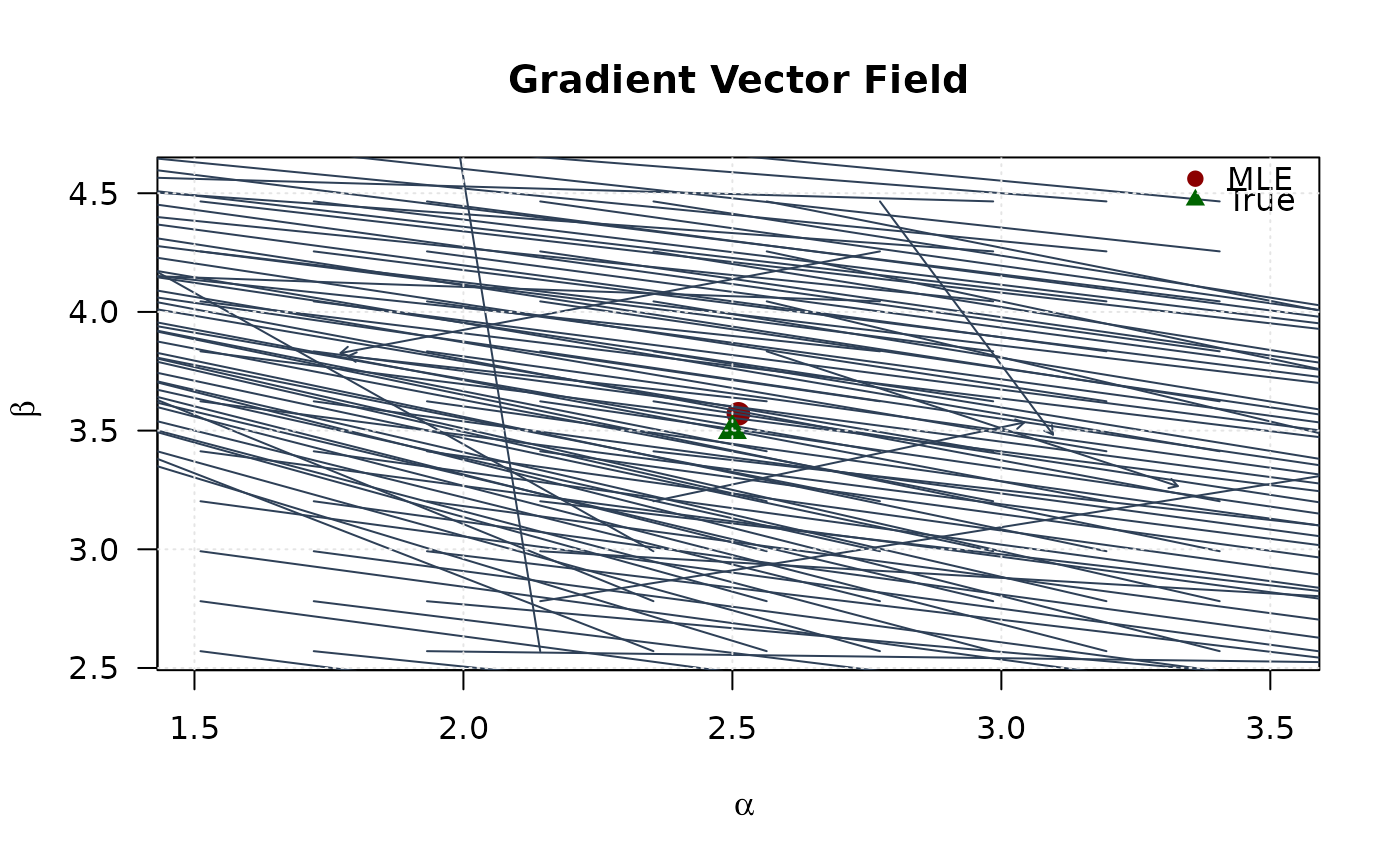
## Example 5: Gradient Path Visualization
# Create grid
alpha_grid <- seq(mle[1] - 1, mle[1] + 1, length.out = 20)
beta_grid <- seq(mle[2] - 1, mle[2] + 1, length.out = 20)
alpha_grid <- alpha_grid[alpha_grid > 0]
beta_grid <- beta_grid[beta_grid > 0]
# Compute gradient vectors
grad_alpha <- matrix(NA, nrow = length(alpha_grid), ncol = length(beta_grid))
grad_beta <- matrix(NA, nrow = length(alpha_grid), ncol = length(beta_grid))
for (i in seq_along(alpha_grid)) {
for (j in seq_along(beta_grid)) {
g <- grkw(c(alpha_grid[i], beta_grid[j]), data)
grad_alpha[i, j] <- -g[1] # Negative for gradient ascent
grad_beta[i, j] <- -g[2]
}
}
# Plot gradient field
plot(mle[1], mle[2],
pch = 19, col = "#8B0000", cex = 1.5,
xlim = range(alpha_grid), ylim = range(beta_grid),
xlab = expression(alpha), ylab = expression(beta),
main = "Gradient Vector Field", las = 1
)
# Subsample for clearer visualization
step <- 2
for (i in seq(1, length(alpha_grid), by = step)) {
for (j in seq(1, length(beta_grid), by = step)) {
arrows(alpha_grid[i], beta_grid[j],
alpha_grid[i] + 0.05 * grad_alpha[i, j],
beta_grid[j] + 0.05 * grad_beta[i, j],
length = 0.05, col = "#2E4057", lwd = 1
)
}
}
points(true_params[1], true_params[2], pch = 17, col = "#006400", cex = 1.5)
legend("topright",
legend = c("MLE", "True"),
col = c("#8B0000", "#006400"),
pch = c(19, 17), bty = "n"
)
grid(col = "gray90")
 ## Example 6: Score Test Statistic
# Score test for H0: theta = theta0
theta0 <- c(2, 3)
score_theta0 <- -grkw(par = theta0, data = data) # Score is negative gradient
# Fisher information at theta0 (using Hessian)
fisher_info <- hskw(par = theta0, data = data)
# Score test statistic
score_stat <- t(score_theta0) %*% solve(fisher_info) %*% score_theta0
p_value <- pchisq(score_stat, df = 2, lower.tail = FALSE)
cat("\nScore Test:\n")
#>
#> Score Test:
cat("H0: alpha = 2, beta = 3\n")
#> H0: alpha = 2, beta = 3
cat("Score vector:", score_theta0, "\n")
#> Score vector: 170.1849 -42.66137
cat("Test statistic:", score_stat, "\n")
#> Test statistic: 55.14706
cat("P-value:", format.pval(p_value, digits = 4), "\n")
#> P-value: 1.059e-12
# }
## Example 6: Score Test Statistic
# Score test for H0: theta = theta0
theta0 <- c(2, 3)
score_theta0 <- -grkw(par = theta0, data = data) # Score is negative gradient
# Fisher information at theta0 (using Hessian)
fisher_info <- hskw(par = theta0, data = data)
# Score test statistic
score_stat <- t(score_theta0) %*% solve(fisher_info) %*% score_theta0
p_value <- pchisq(score_stat, df = 2, lower.tail = FALSE)
cat("\nScore Test:\n")
#>
#> Score Test:
cat("H0: alpha = 2, beta = 3\n")
#> H0: alpha = 2, beta = 3
cat("Score vector:", score_theta0, "\n")
#> Score vector: 170.1849 -42.66137
cat("Test statistic:", score_stat, "\n")
#> Test statistic: 55.14706
cat("P-value:", format.pval(p_value, digits = 4), "\n")
#> P-value: 1.059e-12
# }