Computes the analytic 2x2 Hessian matrix (matrix of second partial derivatives)
of the negative log-likelihood function for the two-parameter Kumaraswamy (Kw)
distribution with parameters alpha (\(\alpha\)) and beta
(\(\beta\)). The Hessian is useful for estimating standard errors and in
optimization algorithms.
Value
Returns a 2x2 numeric matrix representing the Hessian matrix of the
negative log-likelihood function, \(-\partial^2 \ell / (\partial \theta_i \partial \theta_j)\),
where \(\theta = (\alpha, \beta)\).
Returns a 2x2 matrix populated with NaN if any parameter values are
invalid according to their constraints, or if any value in data is
not in the interval (0, 1).
Details
This function calculates the analytic second partial derivatives of the
negative log-likelihood function (\(-\ell(\theta|\mathbf{x})\)). The components
are the negative of the second derivatives of the log-likelihood \(\ell\)
(derived from the PDF in dkw).
Let \(v_i = 1 - x_i^{\alpha}\). The second derivatives of the positive log-likelihood (\(\ell\)) are: $$ \frac{\partial^2 \ell}{\partial \alpha^2} = -\frac{n}{\alpha^2} - (\beta-1)\sum_{i=1}^{n}\frac{x_i^{\alpha}(\ln(x_i))^2}{v_i^2} $$ $$ \frac{\partial^2 \ell}{\partial \alpha \partial \beta} = - \sum_{i=1}^{n}\frac{x_i^{\alpha}\ln(x_i)}{v_i} $$ $$ \frac{\partial^2 \ell}{\partial \beta^2} = -\frac{n}{\beta^2} $$ The function returns the Hessian matrix containing the negative of these values.
Key properties of the returned matrix:
Dimensions: 2x2.
Symmetry: The matrix is symmetric.
Ordering: Rows and columns correspond to the parameters in the order \(\alpha, \beta\).
Content: Analytic second derivatives of the negative log-likelihood.
This corresponds to the relevant 2x2 submatrix of the 5x5 GKw Hessian (hsgkw)
evaluated at \(\gamma=1, \delta=0, \lambda=1\).
References
Kumaraswamy, P. (1980). A generalized probability density function for double-bounded random processes. Journal of Hydrology, 46(1-2), 79-88.
Jones, M. C. (2009). Kumaraswamy's distribution: A beta-type distribution with some tractability advantages. Statistical Methodology, 6(1), 70-81.
(Note: Specific Hessian formulas might be derived or sourced from additional references).
Examples
# \donttest{
## Example 1: Basic Hessian Evaluation
# Generate sample data
set.seed(123)
n <- 1000
true_params <- c(alpha = 2.5, beta = 3.5)
data <- rkw(n, alpha = true_params[1], beta = true_params[2])
# Evaluate Hessian at true parameters
hess_true <- hskw(par = true_params, data = data)
cat("Hessian matrix at true parameters:\n")
#> Hessian matrix at true parameters:
print(hess_true, digits = 4)
#> [,1] [,2]
#> [1,] 449.7 -153.72
#> [2,] -153.7 81.63
# Check symmetry
cat(
"\nSymmetry check (max |H - H^T|):",
max(abs(hess_true - t(hess_true))), "\n"
)
#>
#> Symmetry check (max |H - H^T|): 0
## Example 2: Hessian Properties at MLE
# Fit model
fit <- optim(
par = c(2, 2),
fn = llkw,
gr = grkw,
data = data,
method = "BFGS",
hessian = TRUE
)
mle <- fit$par
names(mle) <- c("alpha", "beta")
# Hessian at MLE
hessian_at_mle <- hskw(par = mle, data = data)
cat("\nHessian at MLE:\n")
#>
#> Hessian at MLE:
print(hessian_at_mle, digits = 4)
#> [,1] [,2]
#> [1,] 453.2 -152.43
#> [2,] -152.4 78.43
# Compare with optim's numerical Hessian
cat("\nComparison with optim Hessian:\n")
#>
#> Comparison with optim Hessian:
cat(
"Max absolute difference:",
max(abs(hessian_at_mle - fit$hessian)), "\n"
)
#> Max absolute difference: 8.859183e-05
# Eigenvalue analysis
eigenvals <- eigen(hessian_at_mle, only.values = TRUE)$values
cat("\nEigenvalues:\n")
#>
#> Eigenvalues:
print(eigenvals)
#> [1] 507.36836 24.25944
cat("\nPositive definite:", all(eigenvals > 0), "\n")
#>
#> Positive definite: TRUE
cat("Condition number:", max(eigenvals) / min(eigenvals), "\n")
#> Condition number: 20.91426
## Example 3: Standard Errors and Confidence Intervals
# Observed information matrix (negative Hessian for neg-loglik)
obs_info <- hessian_at_mle
# Variance-covariance matrix
vcov_matrix <- solve(obs_info)
cat("\nVariance-Covariance Matrix:\n")
#>
#> Variance-Covariance Matrix:
print(vcov_matrix, digits = 6)
#> [,1] [,2]
#> [1,] 0.0063718 0.0123841
#> [2,] 0.0123841 0.0368202
# Standard errors
se <- sqrt(diag(vcov_matrix))
names(se) <- c("alpha", "beta")
# Correlation matrix
corr_matrix <- cov2cor(vcov_matrix)
cat("\nCorrelation Matrix:\n")
#>
#> Correlation Matrix:
print(corr_matrix, digits = 4)
#> [,1] [,2]
#> [1,] 1.0000 0.8085
#> [2,] 0.8085 1.0000
# Confidence intervals
z_crit <- qnorm(0.975)
results <- data.frame(
Parameter = c("alpha", "beta"),
True = true_params,
MLE = mle,
SE = se,
CI_Lower = mle - z_crit * se,
CI_Upper = mle + z_crit * se
)
print(results, digits = 4)
#> Parameter True MLE SE CI_Lower CI_Upper
#> alpha alpha 2.5 2.511 0.07982 2.355 2.668
#> beta beta 3.5 3.571 0.19189 3.195 3.947
## Example 4: Determinant and Trace Analysis
# Compute at different points
test_params <- rbind(
c(1.5, 2.5),
c(2.0, 3.0),
mle,
c(3.0, 4.0)
)
hess_properties <- data.frame(
Alpha = numeric(),
Beta = numeric(),
Determinant = numeric(),
Trace = numeric(),
Min_Eigenval = numeric(),
Max_Eigenval = numeric(),
Cond_Number = numeric(),
stringsAsFactors = FALSE
)
for (i in 1:nrow(test_params)) {
H <- hskw(par = test_params[i, ], data = data)
eigs <- eigen(H, only.values = TRUE)$values
hess_properties <- rbind(hess_properties, data.frame(
Alpha = test_params[i, 1],
Beta = test_params[i, 2],
Determinant = det(H),
Trace = sum(diag(H)),
Min_Eigenval = min(eigs),
Max_Eigenval = max(eigs),
Cond_Number = max(eigs) / min(eigs)
))
}
cat("\nHessian Properties at Different Points:\n")
#>
#> Hessian Properties at Different Points:
print(hess_properties, digits = 4, row.names = FALSE)
#> Alpha Beta Determinant Trace Min_Eigenval Max_Eigenval Cond_Number
#> 1.500 2.500 27209 1185.6 23.41 1162.2 49.64
#> 2.000 3.000 19189 760.5 26.13 734.3 28.10
#> 2.511 3.571 12308 531.6 24.26 507.4 20.91
#> 3.000 4.000 8945 391.2 24.39 366.8 15.04
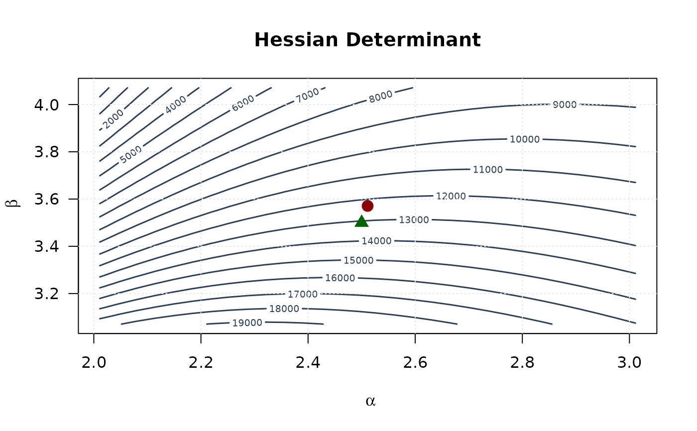
## Example 5: Curvature Visualization
# Create grid around MLE
alpha_grid <- seq(mle[1] - 0.5, mle[1] + 0.5, length.out = 30)
beta_grid <- seq(mle[2] - 0.5, mle[2] + 0.5, length.out = 30)
alpha_grid <- alpha_grid[alpha_grid > 0]
beta_grid <- beta_grid[beta_grid > 0]
# Compute curvature measures
determinant_surface <- matrix(NA,
nrow = length(alpha_grid),
ncol = length(beta_grid)
)
trace_surface <- matrix(NA,
nrow = length(alpha_grid),
ncol = length(beta_grid)
)
for (i in seq_along(alpha_grid)) {
for (j in seq_along(beta_grid)) {
H <- hskw(c(alpha_grid[i], beta_grid[j]), data)
determinant_surface[i, j] <- det(H)
trace_surface[i, j] <- sum(diag(H))
}
}
# Plot
contour(alpha_grid, beta_grid, determinant_surface,
xlab = expression(alpha), ylab = expression(beta),
main = "Hessian Determinant", las = 1,
col = "#2E4057", lwd = 1.5, nlevels = 15
)
points(mle[1], mle[2], pch = 19, col = "#8B0000", cex = 1.5)
points(true_params[1], true_params[2], pch = 17, col = "#006400", cex = 1.5)
grid(col = "gray90")
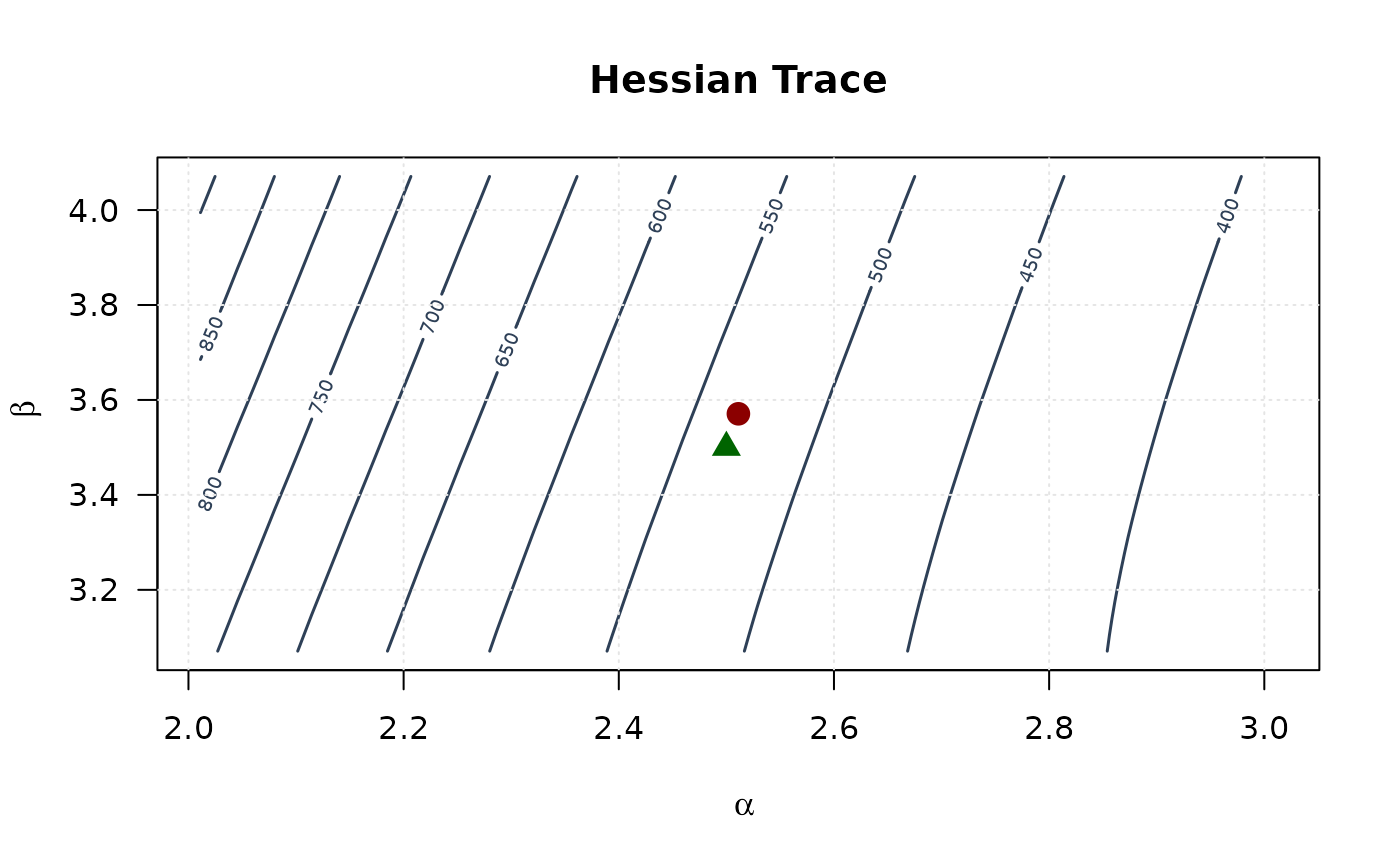
 contour(alpha_grid, beta_grid, trace_surface,
xlab = expression(alpha), ylab = expression(beta),
main = "Hessian Trace", las = 1,
col = "#2E4057", lwd = 1.5, nlevels = 15
)
points(mle[1], mle[2], pch = 19, col = "#8B0000", cex = 1.5)
points(true_params[1], true_params[2], pch = 17, col = "#006400", cex = 1.5)
grid(col = "gray90")
contour(alpha_grid, beta_grid, trace_surface,
xlab = expression(alpha), ylab = expression(beta),
main = "Hessian Trace", las = 1,
col = "#2E4057", lwd = 1.5, nlevels = 15
)
points(mle[1], mle[2], pch = 19, col = "#8B0000", cex = 1.5)
points(true_params[1], true_params[2], pch = 17, col = "#006400", cex = 1.5)
grid(col = "gray90")
 ## Example 6: Fisher Information and Asymptotic Efficiency
# Observed information (at MLE)
obs_fisher <- hessian_at_mle
# Asymptotic covariance matrix
asymp_cov <- solve(obs_fisher)
cat("\nAsymptotic Standard Errors:\n")
#>
#> Asymptotic Standard Errors:
cat("SE(alpha):", sqrt(asymp_cov[1, 1]), "\n")
#> SE(alpha): 0.07982353
cat("SE(beta):", sqrt(asymp_cov[2, 2]), "\n")
#> SE(beta): 0.191886
# Cramér-Rao Lower Bound
cat("\nCramér-Rao Lower Bounds:\n")
#>
#> Cramér-Rao Lower Bounds:
cat("CRLB(alpha):", sqrt(asymp_cov[1, 1]), "\n")
#> CRLB(alpha): 0.07982353
cat("CRLB(beta):", sqrt(asymp_cov[2, 2]), "\n")
#> CRLB(beta): 0.191886
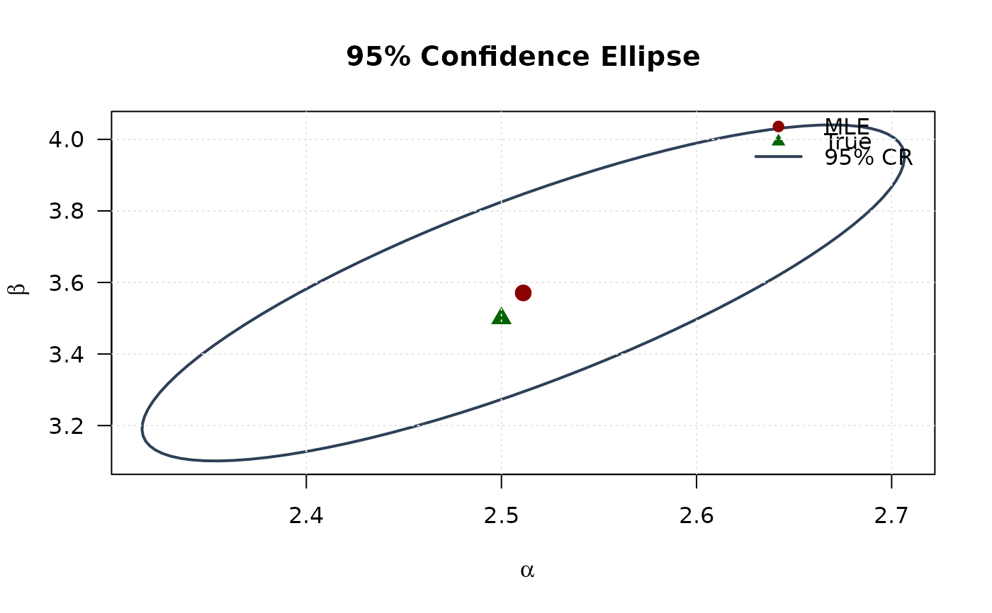
# Efficiency ellipse (95% confidence region)
theta <- seq(0, 2 * pi, length.out = 100)
chi2_val <- qchisq(0.95, df = 2)
# Eigendecomposition
eig_decomp <- eigen(asymp_cov)
# Ellipse points
ellipse <- matrix(NA, nrow = 100, ncol = 2)
for (i in 1:100) {
v <- c(cos(theta[i]), sin(theta[i]))
ellipse[i, ] <- mle + sqrt(chi2_val) *
(eig_decomp$vectors %*% diag(sqrt(eig_decomp$values)) %*% v)
}
# Plot confidence ellipse
plot(ellipse[, 1], ellipse[, 2],
type = "l", lwd = 2, col = "#2E4057",
xlab = expression(alpha), ylab = expression(beta),
main = "95% Confidence Ellipse", las = 1
)
points(mle[1], mle[2], pch = 19, col = "#8B0000", cex = 1.5)
points(true_params[1], true_params[2], pch = 17, col = "#006400", cex = 1.5)
legend("topright",
legend = c("MLE", "True", "95% CR"),
col = c("#8B0000", "#006400", "#2E4057"),
pch = c(19, 17, NA), lty = c(NA, NA, 1),
lwd = c(NA, NA, 2), bty = "n"
)
grid(col = "gray90")
## Example 6: Fisher Information and Asymptotic Efficiency
# Observed information (at MLE)
obs_fisher <- hessian_at_mle
# Asymptotic covariance matrix
asymp_cov <- solve(obs_fisher)
cat("\nAsymptotic Standard Errors:\n")
#>
#> Asymptotic Standard Errors:
cat("SE(alpha):", sqrt(asymp_cov[1, 1]), "\n")
#> SE(alpha): 0.07982353
cat("SE(beta):", sqrt(asymp_cov[2, 2]), "\n")
#> SE(beta): 0.191886
# Cramér-Rao Lower Bound
cat("\nCramér-Rao Lower Bounds:\n")
#>
#> Cramér-Rao Lower Bounds:
cat("CRLB(alpha):", sqrt(asymp_cov[1, 1]), "\n")
#> CRLB(alpha): 0.07982353
cat("CRLB(beta):", sqrt(asymp_cov[2, 2]), "\n")
#> CRLB(beta): 0.191886
# Efficiency ellipse (95% confidence region)
theta <- seq(0, 2 * pi, length.out = 100)
chi2_val <- qchisq(0.95, df = 2)
# Eigendecomposition
eig_decomp <- eigen(asymp_cov)
# Ellipse points
ellipse <- matrix(NA, nrow = 100, ncol = 2)
for (i in 1:100) {
v <- c(cos(theta[i]), sin(theta[i]))
ellipse[i, ] <- mle + sqrt(chi2_val) *
(eig_decomp$vectors %*% diag(sqrt(eig_decomp$values)) %*% v)
}
# Plot confidence ellipse
plot(ellipse[, 1], ellipse[, 2],
type = "l", lwd = 2, col = "#2E4057",
xlab = expression(alpha), ylab = expression(beta),
main = "95% Confidence Ellipse", las = 1
)
points(mle[1], mle[2], pch = 19, col = "#8B0000", cex = 1.5)
points(true_params[1], true_params[2], pch = 17, col = "#006400", cex = 1.5)
legend("topright",
legend = c("MLE", "True", "95% CR"),
col = c("#8B0000", "#006400", "#2E4057"),
pch = c(19, 17, NA), lty = c(NA, NA, 1),
lwd = c(NA, NA, 2), bty = "n"
)
grid(col = "gray90")
 # }
# }