
Expected loss and regulatory capital
Source:vignettes/articles/expected-loss-and-capital.Rmd
expected-loss-and-capital.RmdThis is the third of three articles on the IRB risk parameters. PD calibration and rating
grades builds the probability of default and LGD and EAD under IRB the loss
given default and the exposure at default, both starting from the
scorecard pipeline of Get
started. This article turns the three parameters into expected loss,
IRB risk weights, capital with the output floor and accounting ECL. It
works on the bundled scr_demo_portfolio, whose PD, LGD and
EAD columns are of the kind those models produce (grade PDs, pool LGDs,
exposures), rather than on the objects built there, so that the
portfolio can cover six asset classes at once.
The regulatory texts behind the parameter tables are listed in scr_irb_params().
Regulation changes and each supervisor interprets it: check the tables
against the texts in force before any regulatory use.
library(scorecraft)
library(data.table)
cfg <- scr_config(verbose = FALSE, nthread = 2)
1. Expected and unexpected loss
The loss a portfolio produces in an average year is its
expected loss, EL = PD * LGD * EAD; it is
a cost of doing business and is covered by provisions and pricing. The
loss in a bad year exceeds that average, and the gap between a high
quantile of the loss distribution and its mean is the unexpected
loss that capital must absorb. The IRB risk-weight function
turns a through-the-cycle PD into the PD of a year at the 99.9% quantile
of a one-factor model, and charges capital for the difference between
the loss at that quantile and the expected loss. Every number that a
regime fixes in that calculation (PD and LGD floors, asset correlations,
the maturity rule, the confidence level, the standardized risk weights
that the output floor compares against) lives in a table returned by
scr_irb_params() and selected by a preset; nothing is
hard-coded in the functions that consume it, and an edited table is
recorded as such on every object built from it.
2. The parameter tables
scr_irb_params() returns every regime-specific number as
a table; the print summarizes them.
p <- scr_irb_params("bcb")
p
#> <scr_irb_params> framework: bcb
#>   BCB Resolutions 303/2023 (IRB) and 229/2022 (standardized); values as tables, editable
#>   PD floors:   corporate 0.05% | bank 0.05% | sovereign none | retail_mortgage 0.05% | qrre_transactor 0.05% | qrre_revolver 0.10% | retail_other 0.05%
#>   LGD floors (unsecured):  corporate 25% | retail_mortgage n/a | qrre 50% | retail_other 30%
#>   F-IRB LGD: senior_unsecured 75% | priority_claim 45% | subordinated 75% | secured_financial 0% | secured_receivables 20% | secured_real_estate 20% | secured_other 25%
#>   CCF (standardized): uncond_cancellable 10% | commitment 40% | nif_ruf 50% | direct_substitute 100% | own-estimate floor 50% of the standardized value
#>   correlation: corporate 0.12-0.24 (k=50) | mortgage 0.15 | QRRE 0.04 | other retail 0.03-0.16 (k=35) | FI x1.25 | SME adj 0.04 (BRL m 15-300)
#>   confidence 0.999 | scaling factor 1 | M default 2.5 in [1, 5] | output floor 72.5% | SA risk weights: 26 rows
p$pd_floor
#>        asset_class floor
#>             <char> <num>
#> 1:       corporate 5e-04
#> 2:            bank 5e-04
#> 3:       sovereign    NA
#> 4: retail_mortgage 5e-04
#> 5: qrre_transactor 5e-04
#> 6:   qrre_revolver 1e-03
#> 7:    retail_other 5e-04
There are three presets. "bcb" takes its values from BCB
Resolution 303/2023, "basel3_final" from the consolidated
Basel Framework, whose CRE31 chapter is the risk-weight function, and
"crr3" from the EU Capital Requirements Regulation as
amended in 2024; "crr3" currently carries the same tables
as "basel3_final". Between "bcb" and
"basel3_final" the visible differences are the supervisory
LGD table of the foundation approach (the "bcb" preset
carries 75% for a senior unsecured claim and 45% for a claim with
priority; the Basel table separates corporates, 40%, from financial
institutions, 45%) and the firm-size bounds of the SME correlation
adjustment. Each table is a default to be checked against the text in
force, not a citation.
p_b3 <- scr_irb_params("basel3_final")
rbind(cbind(framework = "bcb", p$lgd_firb), cbind(framework = "basel3_final", p_b3$lgd_firb))
#>        framework                      claim   lgd
#>           <char>                     <char> <num>
#>  1:          bcb           senior_unsecured  0.75
#>  2:          bcb             priority_claim  0.45
#>  3:          bcb               subordinated  0.75
#>  4:          bcb          secured_financial  0.00
#>  5:          bcb        secured_receivables  0.20
#>  6:          bcb        secured_real_estate  0.20
#>  7:          bcb              secured_other  0.25
#>  8: basel3_final senior_unsecured_corporate  0.40
#>  9: basel3_final        senior_unsecured_fi  0.45
#> 10: basel3_final               subordinated  0.75
#> 11: basel3_final          secured_financial  0.00
#> 12: basel3_final        secured_receivables  0.20
#> 13: basel3_final        secured_real_estate  0.20
#> 14: basel3_final              secured_other  0.25
rbindlist(list(c(framework = "bcb", p$correlation$sme), c(framework = "basel3_final", p_b3$correlation$sme)))
#>       framework    lo    hi   adj   unit
#>          <char> <num> <num> <num> <char>
#> 1:          bcb    15   300  0.04  BRL m
#> 2: basel3_final     5    50  0.04  EUR m
Any cell can be edited and the object passed back through
params; the function that receives it flags
params_modified in its model card.
3. One exposure: scr_el() and
scr_irb_rw()
Expected loss is the primitive. Defaulted exposures replace
PD * LGD with the best estimate of expected loss,
ELBE.
scr_el(c(0.01, 0.02), 0.45, c(1000, 2000))
#> [1]  4.5 18.0
scr_el(0.02, 0.45, 1000, defaulted = TRUE, elbe = 0.6)
#> [1] 600
scr_irb_rw() returns the intermediate quantities of the
risk-weight function, not only the answer: the PD and LGD after floors,
the maturity after clipping, the correlation r, the
maturity adjustment ma and the capital requirement
k. A corporate exposure at PD 1%, LGD 45% and maturity 2.5
years carries a risk weight of 92.32%.
scr_irb_rw(0.01, 0.45, m = 2.5, asset_class = "corporate", params = p)
#>    pd_used lgd_used     m         r         b      ma          k       rw
#>      <num>    <num> <num>     <num>     <num>   <num>      <num>    <num>
#> 1:    0.01     0.45   2.5 0.1927837 0.1374861 1.25981 0.07385344 0.923168
#>         rwa
#>       <num>
#> 1: 0.923168
rbind(
  mortgage     = scr_irb_rw(0.01, 0.20, asset_class = "retail_mortgage", params = p),
  qrre         = scr_irb_rw(0.02, 0.80, asset_class = "qrre_revolver", params = p),
  retail_other = scr_irb_rw(0.02, 0.50, asset_class = "retail_other", params = p)
)[, .(pd_used, lgd_used, r, k, rw)]
#>    pd_used lgd_used          r          k        rw
#>      <num>    <num>      <num>      <num>     <num>
#> 1:    0.01      0.2 0.15000000 0.02005295 0.2506619
#> 2:    0.02      0.8 0.04000000 0.04113480 0.5141850
#> 3:    0.02      0.5 0.09455609 0.05154350 0.6442938
Retail classes have no maturity adjustment (b is
NA, ma is one), so for them K is
exactly LGD times the distance between the stressed and the
unconditional PD. scr_pd_stress() is that stressed PD, and
at q = 0.999 with the regulatory correlation it reproduces
k to machine precision.
o <- scr_irb_rw(0.02, 0.50, asset_class = "retail_other", params = p)
c(k = o$k, by_hand = 0.5 * (scr_pd_stress(0.02, o$r, 0.999) - 0.02))
#>         k   by_hand
#> 0.0515435 0.0515435
scr_pd_stress(0.02, rho = 0.15, q = c(0.5, 0.95, 0.99, 0.999))
#> [1] 0.01295348 0.06219237 0.10558734 0.17632894
The shape of the function differs by asset class because the correlation does: fixed for mortgages (0.15) and revolving retail (0.04), decreasing in PD for corporates and other retail. Plotted at a common LGD of 45%:
grid <- exp(seq(log(1e-4), log(0.3), length.out = 80))
classes <- c("corporate", "retail_mortgage", "qrre_revolver", "retail_other")
curves <- lapply(classes, function(a) scr_irb_rw(grid, 0.45, asset_class = a, params = p)$rw)
plot(grid, curves[[1]], type = "n", log = "x", ylim = c(0, max(unlist(curves))),
     xlab = "PD (log scale)", ylab = "risk weight", main = "IRB risk weight by PD, LGD 45%")
for (i in seq_along(classes)) lines(grid, curves[[i]], lwd = 2, col = i)
legend("topleft", classes, col = seq_along(classes), lwd = 2, bty = "n")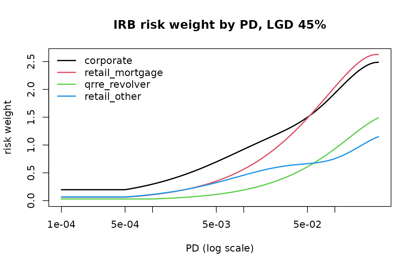
The flat start of every curve is the PD floor: below it the risk
weight no longer falls with the PD. The floors_hit
attribute counts the rows where each floor was binding, and
apply_floors = FALSE shows what the function would return
without them.
r_floored <- scr_irb_rw(grid, 0.45, asset_class = "retail_other", params = p)
attr(r_floored, "floors_hit")
#>        floor     n
#>       <char> <int>
#> 1:  pd_floor    16
#> 2: lgd_floor     0
#> 3:   m_floor     0
#> 4:     m_cap     0
r_raw <- scr_irb_rw(grid, 0.45, asset_class = "retail_other", params = p, apply_floors = FALSE)
data.table(pd = grid, rw_floored = r_floored$rw, rw_no_floor = r_raw$rw)[pd < 6e-4][c(1, 5, 10, 15)]
#>              pd rw_floored rw_no_floor
#>           <num>      <num>       <num>
#> 1: 0.0001000000 0.06629119  0.01834523
#> 2: 0.0001499881 0.06629119  0.02554640
#> 3: 0.0002489589 0.06629119  0.03839309
#> 4: 0.0004132365 0.06629119  0.05720678
# LGD floors: an unsecured own estimate of 10% is lifted to the floor of its class,
# except for the mortgage, whose 5% floor does not bind
scr_irb_rw(0.01, 0.10, asset_class = c("retail_other", "qrre_revolver", "corporate", "retail_mortgage"), params = p)$lgd_used
#> [1] 0.30 0.50 0.25 0.10
# secured by real estate, the retail floor is 10% instead of the unsecured 30%
scr_irb_rw(0.01, 0.05, asset_class = "retail_other", collateral = "real_estate", params = p)$lgd_used
#> [1] 0.1
4. The standardized comparison
The output floor compares the IRB result with a fraction of what the
standardized approach would require, so the same book needs a
standardized risk weight per exposure. scr_sa_rw() looks it
up in params$sa_rw: regulatory retail, mortgages by
loan-to-value band, corporates by rating bucket or the SME weight,
defaulted exposures by provision ratio.
scr_sa_rw(c("retail_other", "retail_mortgage", "retail_mortgage", "corporate", "corporate", "corporate_sme"),
          ltv = c(NA, 0.55, 0.95, NA, NA, NA), rating = c(NA, NA, NA, "A+", NA, NA))
#> [1] 0.75 0.25 0.50 0.50 1.00 0.85
scr_sa_rw("retail_other", defaulted = TRUE, provision_ratio = c(0.1, 0.3))
#> [1] 1.5 1.0
p$sa_rw[asset_class == "retail_mortgage" & sub_class == "standard"]
#>        asset_class sub_class ltv_lo ltv_hi    rw
#>             <char>    <char>  <num>  <num> <num>
#> 1: retail_mortgage  standard    0.0    0.5  0.20
#> 2: retail_mortgage  standard    0.5    0.6  0.25
#> 3: retail_mortgage  standard    0.6    0.8  0.30
#> 4: retail_mortgage  standard    0.8    0.9  0.40
#> 5: retail_mortgage  standard    0.9    1.0  0.50
#> 6: retail_mortgage  standard    1.0    Inf  0.70
5. The portfolio: scr_capital()
scr_demo_portfolio holds 5,000 exposures in six segments
that map one to one onto the asset classes; PD is a grade PD and LGD a
pool value, so segment by grade is homogeneous in PD and LGD, while
maturity varies inside the corporate pools (section 6 comes back to
this). About 3% of the rows are in default with an elbe and
a provision. The whole book is run under the advanced approach
(capital_approach = "airb", the default) to show every
input at work; under the final Basel framework and CRR3 a book of large
corporates would be restricted to the foundation approach, shown at the
end of this section.
d <- scr_demo_portfolio
table(d$segment, d$asset_class)
#>
#>                    corporate corporate_sme qrre_revolver qrre_transactor
#>   cards_revolver           0             0           800               0
#>   cards_transactor         0             0             0             500
#>   corporate_large        500             0             0               0
#>   corporate_sme            0           700             0               0
#>   mortgages                0             0             0               0
#>   retail_loans             0             0             0               0
#>
#>                    retail_mortgage retail_other
#>   cards_revolver                 0            0
#>   cards_transactor               0            0
#>   corporate_large                0            0
#>   corporate_sme                  0            0
#>   mortgages                   1000            0
#>   retail_loans                   0         1500
cap <- scr_capital(d, segment = "segment", asset_class = "asset_class", m = "m",
                   defaulted = "defaulted", elbe = "elbe", provisions = "provision",
                   ltv = "ltv", rating = "rating", sales = "sales", transactor = "transactor",
                   grade = "grade", id = "id", config = cfg, keep_rows = TRUE)
cap
#> <scr_capital> bcb | airb | 5,000 exposures in 6 segments
#>   EAD 1,940,402,792 | EL 31,028,477 (1.60%) | RWA IRB 1,214,315,257 | density 62.6% | capital (8.0%) 97,145,221
#>   standardized RWA 1,553,528,212 | IRB/SA 0.782 | output floor 72.5%: not binding (headroom 88,007,303)
#>   provisions 43,425,571 vs EL: shortfall 0 | excess 12,397,094 | tier 2 add-back 7,285,892 (cap 7,285,892)
#>   floors: pd 194 rows, RWA 5,221,058 | lgd 0 rows, RWA         0 | m 0 rows, RWA         0 | HHI 0.00231 (n_eff 433, max share 1.19%)
#>   top segments by RWA:
#>     corporate_large        n 500     EAD 1,451,911,238  RW  65.1%  RWA 944,938,904     IRB/SA 0.77
#>     corporate_sme          n 700     EAD 302,516,540    RW  79.2%  RWA 239,492,431     IRB/SA 0.92
#>     mortgages              n 1,000   EAD 165,305,905    RW  12.6%  RWA 20,764,980      IRB/SA 0.37
#>     retail_loans           n 1,500   EAD 15,592,011     RW  44.5%  RWA 6,935,236       IRB/SA 0.59
#>     cards_revolver         n 800     EAD 3,282,347      RW  54.2%  RWA 1,777,936       IRB/SA 0.71
#>   sensitivity: vasicek_q0.99 +95.8% | vasicek_q0.95 +55.7% | r_x1.25 +26.8%
Totals and the reconciliation by segment
Every figure on the print is in cap$totals, and
cap$segments breaks it down: EAD-weighted inputs, the IRB
and standardized risk-weighted assets side by side, expected loss and
provisions.
with(cap$totals, data.table(ead, el, el_rate, rwa_irb, rwa_sa, irb_sa_ratio, density, capital))
#>           ead       el    el_rate    rwa_irb     rwa_sa irb_sa_ratio   density
#>         <num>    <num>      <num>      <num>      <num>        <num>     <num>
#> 1: 1940402792 31028477 0.01599074 1214315257 1553528212      0.78165 0.6258058
#>     capital
#>       <num>
#> 1: 97145221
cap$segments[, .(segment, n, ead, pd_mean, lgd_mean, rw, rwa_irb, irb_sa_ratio, el, provisions, shortfall_excess)]
#>             segment     n        ead    pd_mean lgd_mean        rw     rwa_irb
#>              <char> <int>      <num>      <num>    <num>     <num>       <num>
#> 1:  corporate_large   500 1451911238 0.03359715     0.40 0.6508242 944938904.4
#> 2:    corporate_sme   700  302516540 0.06973651     0.42 0.7916672 239492431.3
#> 3:        mortgages  1000  165305905 0.01792392     0.15 0.1256155  20764979.8
#> 4:     retail_loans  1500   15592011 0.05400681     0.45 0.4447942   6935236.3
#> 5:   cards_revolver   800    3282347 0.07501589     0.75 0.5416660   1777935.7
#> 6: cards_transactor   500    1794751 0.03000090     0.70 0.2260868    405769.5
#>    irb_sa_ratio         el provisions shortfall_excess
#>           <num>      <num>      <num>            <num>
#> 1:    0.7729808 20926478.3   30840652      9914173.739
#> 2:    0.9233544  9087003.5   10039600       952596.493
#> 3:    0.3672066   421450.8    1963358      1541907.188
#> 4:    0.5866356   374260.3     396848        22587.723
#> 5:    0.7118514   181708.6     142177       -39531.608
#> 6:    0.4907211    37575.5      42936         5360.503
The irb_sa_ratio column says where the IRB approach
saves the most against the standardized one; mortgages sit far below the
72.5% line on their own, the large corporate book just above it and the
SME book well above, and the output floor is applied to the total, not
by segment. The total here is credit risk only: the regulatory floor
compares the whole of the risk-weighted assets, market and operational
risk included, with 72.5% of their standardized counterparts, so the
figure below is a credit-portfolio view of the floor, not the
bank’s.
Floors and the output-floor bridge
cap$floors measures each input floor by the rows it
binds, their EAD and the risk-weighted assets it adds. Here only the PD
floor bites (the two safest grades start below it on purpose), and the
bridge from the unfloored IRB figure to the reported one reads:
cap$floors
#>        floor n_hit   ead_hit delta_rwa
#>       <char> <int>     <num>     <num>
#> 1:  pd_floor   194 110745561   5221058
#> 2: lgd_floor     0         0         0
#> 3:   m_floor     0         0         0
with(cap$totals, data.table(
  step  = c("rwa_irb_no_floors", "input_floors", "rwa_irb", "rwa_sa", "output_floor_rwa", "rwa_reported"),
  value = c(rwa_irb_no_floors, rwa_irb - rwa_irb_no_floors, rwa_irb, rwa_sa, rwa_floor, rwa_reported)))
#>                 step      value
#>               <char>      <num>
#> 1: rwa_irb_no_floors 1209094199
#> 2:      input_floors    5221058
#> 3:           rwa_irb 1214315257
#> 4:            rwa_sa 1553528212
#> 5:  output_floor_rwa 1126307953
#> 6:      rwa_reported 1214315257
with(cap$totals, data.table(floor_binding, headroom))
#>    floor_binding headroom
#>           <lgcl>    <num>
#> 1:         FALSE 88007303
rwa_reported is the larger of the IRB figure and
output_floor * rwa_sa; headroom is the
distance to the floor, negative when it binds.
Expected loss against provisions
Regulatory EL is compared with the provision stock. A shortfall is
deducted from common equity tier 1; an excess counts as tier 2 up to
0.6% of the IRB risk-weighted assets, which is why
tier2_addback can be smaller than excess. The
comparison is made on the totals, defaulted and performing exposures
together. The Basel text (CRE35) and the CRR compare the two separately,
so that an excess of specific provisions on defaulted exposures cannot
cover a shortfall on performing ones; where that distinction matters,
run the function on each part and combine the results.
with(cap$totals, data.table(el, provisions, shortfall, excess, tier2_cap, tier2_addback))
#>          el provisions shortfall   excess tier2_cap tier2_addback
#>       <num>      <num>     <num>    <num>     <num>         <num>
#> 1: 31028477   43425571         0 12397094   7285892       7285892
Sensitivity
The grid re-runs the whole function under fixed shocks. The two
Vasicek rows stress every performing PD with
scr_pd_stress() at the exposure’s own correlation and feed
the stressed PD back into the function, so that the correlation follows
the PD; they are the closest the grid comes to a bad-year capital
figure.
cap$sensitivity
#>             shock        rwa      delta    delta_pct
#>            <char>      <num>      <num>        <num>
#>  1:          base 1214315257          0  0.000000000
#>  2:      pd_x1.10 1256949940   42634684  0.035110062
#>  3:      pd_x1.25 1315374005  101058749  0.083222827
#>  4:      pd_x1.50 1401061020  186745763  0.153786887
#>  5:  lgd_plus_5pp 1380658748  166343491  0.136985424
#>  6:     ead_x1.10 1335746783  121431526  0.100000000
#>  7:      no_floor 1209094199   -5221058 -0.004299591
#>  8:       r_x1.25 1540264244  325948987  0.268422047
#>  9: vasicek_q0.95 1890754479  676439222  0.557054042
#> 10: vasicek_q0.99 2377857720 1163542463  0.958188128
The foundation approach
Under capital_approach = "firb" the LGD is the
supervisory value of the claim type, read from
params$lgd_firb through the claim column, no
LGD floor applies and the maturity is fixed at
params$m_default. The claim names belong to the preset.
Here the large corporates are run as senior unsecured claims under the
two presets and set beside the advanced run of the same rows.
big <- d[d$segment == "corporate_large", ]
cap_firb <- function(framework, claim) {
  big$claim <- claim
  scr_capital(big, segment = "segment", asset_class = "asset_class", m = "m",
              defaulted = "defaulted", elbe = "elbe", sales = "sales", rating = "rating",
              grade = "grade", claim = "claim", params = scr_irb_params(framework),
              config = scr_config(verbose = FALSE, nthread = 2, framework = framework,
                                  capital_approach = "firb"))$totals
}
airb  <- cap$segments[segment == "corporate_large"]
f_bcb <- cap_firb("bcb", "senior_unsecured")
f_b3  <- cap_firb("basel3_final", "senior_unsecured_corporate")
data.table(run = c("airb, own LGD", "firb, bcb preset", "firb, basel3_final preset"),
           rwa_irb = c(airb$rwa_irb, f_bcb$rwa_irb, f_b3$rwa_irb),
           el = c(airb$el, f_bcb$el, f_b3$el))
#>                          run    rwa_irb       el
#>                       <char>      <num>    <num>
#> 1:             airb, own LGD  944938904 20926478
#> 2:          firb, bcb preset 1625968473 25912479
#> 3: firb, basel3_final preset  867183186 20926478
The preset drives the result. With the 40% of the Basel table, equal
to the own LGD of this book, the foundation run is lower than the
advanced one because the maturity is fixed at 2.5 years where the book
averages three, and because the defaulted rows carry no
LGD - ELBE charge under the foundation approach. With the
75% the "bcb" preset carries for a senior unsecured claim,
the risk-weighted assets rise by about 70% and the expected loss by
about a quarter (less than in proportion, because the defaulted rows
keep their ELBE).
6. The same numbers in SQL
The production query does not need a normal quantile: the constants
of every pool (PD, LGD, correlation, K, RW,
all after floors) are computed in R and emitted as a
pool_params CTE, and the exposure table is joined to it on
segment and grade. Defaulted rows use ELBE * EAD and
K = max(0, LGD - ELBE) from their own columns.
sql <- scr_sql(cap, table = "portfolio", dialect = "duckdb")
cat(grep("^-- (CTE|  |NOTE)", sql, value = TRUE), sep = "\n")
#> -- CTE pool_params: PD, LGD, correlation, K and RW per pool, computed in R
#> --   (floors applied; no normal quantile needed at run time).
#> -- CTE exposure_capital: el = pd * lgd * ead, rwa = 12.5 * k * ead per exposure;
#> --   rows with defaulted = 1 use ELBE * ead and K = max(0, LGD - ELBE).
#> -- NOTE: at least one pool is not homogeneous: its constants are EAD-weighted, so
#> --   EL and RWA are exact per pool and approximate per exposure. Pass `grade` for finer pools.
cat(tail(sql, 21), sep = "\n")
#>   SELECT
#>     e.id,
#>     e.segment,
#>     e.grade,
#>     e.ead AS ead,
#>     CASE WHEN e.defaulted = 1 THEN COALESCE(e.elbe, e.lgd) * e.ead ELSE p.pd * p.lgd * e.ead END AS el,
#>     CASE WHEN e.defaulted = 1 THEN (CASE WHEN e.lgd - COALESCE(e.elbe, e.lgd) > 0 THEN e.lgd - COALESCE(e.elbe, e.lgd) ELSE 0 END) ELSE p.k END AS k
#>   FROM portfolio e
#>   JOIN pool_params p ON e.segment = p.segment AND e.grade = p.grade
#> )
#>
#> SELECT
#>     id,
#>     segment,
#>     grade,
#>     ead,
#>     el,
#>     k,
#>     12.5 * k AS rw,
#>     12.5 * k * ead AS rwa
#> FROM exposure_capital;
The retail pools are homogeneous, so the query reproduces R row by row; the corporate pools carry a maturity that varies inside the pool, so their constants are EAD-weighted and the match is exact at pool level (the header of the SQL says so). Both facts can be checked on DuckDB.
con <- DBI::dbConnect(duckdb::duckdb())
DBI::dbWriteTable(con, "portfolio", d)
got <- DBI::dbGetQuery(con, paste(sql, collapse = "\n"))
got <- got[match(d$id, got$id), ]
ex <- cap$exposures
retail <- !d$segment %in% c("corporate_large", "corporate_sme")
data.table(id = d$id, segment = d$segment, el_r = ex$el, el_sql = got$el, rwa_r = ex$rwa, rwa_sql = got$rwa)[retail][1:4]
#>        id        segment      el_r    el_sql     rwa_r   rwa_sql
#>    <char>         <char>     <num>     <num>     <num>     <num>
#> 1: E00001   retail_loans  18.65707  18.65707  2386.003  2386.003
#> 2: E00002      mortgages 256.42922 256.42922 36989.679 36989.679
#> 3: E00003 cards_revolver  99.56714  99.56714  2210.792  2210.792
#> 4: E00004      mortgages  68.02380  68.02380 12261.888 12261.888
c(el = all.equal(got$el[retail], ex$el[retail]), rwa = all.equal(got$rwa[retail], ex$rwa[retail]))
#>   el  rwa
#> TRUE TRUE
agg <- DBI::dbGetQuery(con, paste(scr_sql(cap, table = "portfolio", dialect = "duckdb", level = "portfolio"), collapse = "\n"))
agg <- agg[match(cap$segments$segment, agg$segment), ]
c(rwa = all.equal(agg$rwa, cap$segments$rwa_irb), el = all.equal(agg$el, cap$segments$el))
#>  rwa   el
#> TRUE TRUE
DBI::dbDisconnect(con, shutdown = TRUE)
7. Accounting expected credit loss: scr_ecl()
scr_ecl() computes the discrete-time expected credit
loss: a survival-weighted sum of marginal monthly hazards times LGD and
EAD, discounted at the effective interest rate. With a flat hazard, no
discounting and no prepayment the sum collapses to the closed form
LGD * EAD * (1 - (1 - h)^T).
cfg_none <- scr_config(verbose = FALSE, nthread = 2, ecl_discount = "none")
h <- 0.01; lgd <- 0.4; ead <- 1000
e1 <- scr_ecl(h, lgd, ead, t_max = 36L, config = cfg_none)
c(ecl_12m = e1$totals$ecl_12m, closed_form = lgd * ead * (1 - (1 - h)^12),
  ecl_life = e1$totals$ecl_life, closed_form = lgd * ead * (1 - (1 - h)^36))
#>     ecl_12m closed_form    ecl_life closed_form
#>    45.44605    45.44605   121.43471   121.43471
On the portfolio, the annual grade PD becomes a flat monthly hazard,
run over a term that depends on the product: twenty years for mortgages,
the contractual maturity for corporates and three years for the other
retail lines. The hazard matrix is zero after the term of each row, so
the lifetime figure stops there. The stage is allocated by the rule: 90
days past due for stage 3; 30 days past due, or a 12-month PD at least
twice the one at origination, for stage 2. The 30-day backstop is the
rebuttable presumption of IFRS 9; the ratio of two is a common
convention, set by ecl_sicr_ratio, not a threshold the
standard prescribes. Three scenarios are weighted. The z
shock moves every monthly hazard through the one-factor model with the
correlation rho, given explicitly here because the default
(0.15) is only a placeholder; applied month by month, the shock raises
the 12-month PD more than the same z applied to the annual
PD would. lgd_add and ead_mult do what their
names say.
Two inputs are shortcuts that a real ECL model would not take. The PD
here is a regulatory grade PD, through-the-cycle and possibly carrying a
margin and a floor, and the LGD is a pool value that may include a
downturn component; IFRS 9 asks for unbiased, point-in-time,
forward-looking estimates, such as pd_be mapped to the
current state of the cycle (see the point-in-time section of the PD
article) and an LGD without the downturn and the margin. The mechanics
below are unchanged by that choice; the numbers are not.
hz <- 1 - (1 - d$pd)^(1 / 12)
term <- ifelse(d$segment == "mortgages", 240L,
               ifelse(is.na(d$m), 36L, as.integer(round(12 * d$m))))
hz_term <- outer(hz, rep(1, max(term)))
hz_term[col(hz_term) > term] <- 0
ecl <- scr_ecl(hz_term, d$lgd, d$ead, eir = d$eir, dpd = d$dpd, pd_orig = d$pd_orig,
               rho = 0.10, segment = d$segment, id = d$id,
               scenarios = list(base = list(), downturn = list(z = -1, lgd_add = 0.05), upturn = list(z = 1)),
               weights = c(0.5, 0.3, 0.2), config = cfg)
ecl
#> <scr_ecl> 5,000 exposures | ECL 31,966,351 | coverage 1.65% | 12-month horizon 12 of 240 months | discount: eir
#>   stage rule: dpd >= 90 -> stage 3; dpd >= 30 or PD ratio >= 2 -> stage 2
#>   stage 1  n 4,304   EAD 1,687,138,403  ECL 8,069,792    coverage 0.48%
#>   stage 2  n 542     EAD 201,418,836    ECL 2,429,902    coverage 1.21%
#>   stage 3  n 154     EAD 51,845,553     ECL 21,466,657   coverage 41.41%
#>   12-month 30,524,224 | lifetime 44,113,928 | scenarios: base 0.50, downturn 0.30, upturn 0.20
ecl$scenarios
#>    scenario weight  ecl_12m ecl_life      ecl
#>      <char>  <num>    <num>    <num>    <num>
#> 1:     base    0.5 28846459 41358454 30157406
#> 2: downturn    0.3 38686456 61177845 41134697
#> 3:   upturn    0.2 22475291 25406736 22736196
ecl$stages
#> Key: <stage>
#>    stage     n        ead    ecl_12m ecl_life      ecl    coverage
#>    <int> <int>      <num>      <num>    <num>    <num>       <num>
#> 1:     1  4304 1687138403  8069792.3 20217368  8069792 0.004783124
#> 2:     2   542  201418836   987774.7  2429902  2429902 0.012063925
#> 3:     3   154   51845553 21466657.4 21466657 21466657 0.414050119
Accounting ECL and regulatory EL measure different things and are not
expected to agree: the ECL of stage 2 is a lifetime figure, the ECL of
stage 3 is LGD * EAD rather than ELBE * EAD,
and the scenario weights tilt the accounting number. Laying the two side
by side per segment is nevertheless the first table a reconciliation
asks for.
merge(cap$segments[, .(segment, ead, el_regulatory = el, provisions)],
      ecl$segments[, .(segment, ecl_accounting = ecl, share_stage2, share_stage3)], by = "segment")[order(-ead)]
#>             segment        ead el_regulatory provisions ecl_accounting
#>              <char>      <num>         <num>      <num>          <num>
#> 1:  corporate_large 1451911238    20926478.3   30840652    21178194.33
#> 2:    corporate_sme  302516540     9087003.5   10039600     9497790.04
#> 3:        mortgages  165305905      421450.8    1963358      652546.02
#> 4:     retail_loans   15592011      374260.3     396848      408339.48
#> 5:   cards_revolver    3282347      181708.6     142177      190857.73
#> 6: cards_transactor    1794751       37575.5      42936       38623.76
#>    share_stage2 share_stage3
#>           <num>        <num>
#> 1:    0.0960000   0.02600000
#> 2:    0.1114286   0.04000000
#> 3:    0.1020000   0.01000000
#> 4:    0.1153333   0.03466667
#> 5:    0.1150000   0.05250000
#> 6:    0.0980000   0.01800000
c(el_regulatory = cap$totals$el, ecl_accounting = ecl$totals$ecl, provisions = cap$totals$provisions)
#>  el_regulatory ecl_accounting     provisions
#>       31028477       31966351       43425571
8. Deliverables
scr_export() writes one workbook with the summary, the
configuration and every table of the object, plus the SQL file.
out <- file.path(tempdir(), "scorecraft-capital")
ex <- scr_export(cap, out, stamp = FALSE)
basename(unlist(ex$files))
#> [1] "capital_bcb.xlsx"    "sql_capital_bcb.sql"
openxlsx::getSheetNames(ex$files$xlsx)
#>  [1] "Capital_Summary"         "Capital_Config"
#>  [3] "Segments_Reconciliation" "Pools"
#>  [5] "Floors_Impact"           "Output_Floor_Bridge"
#>  [7] "Sensitivity"             "Concentration"
#>  [9] "EL_vs_Provisions"        "Exposures"
#> [11] "Model_Card"              "Decision_Ledger"
9. The ledger and the model card
Every choice the function made on the caller’s behalf is a row of the ledger: the preset and approach, where the inputs came from, how many rows each floor touched, whether the output floor binds, and the provision comparison. The model card carries the numbers a validator needs to reproduce the run, including whether the parameter tables were edited.
cap$ledger[, .(action, detail)]
#>          action
#>          <char>
#> 1:    framework
#> 2:       inputs
#> 3:       floors
#> 4: output_floor
#> 5:   provisions
#>                                                                                       detail
#>                                                                                       <char>
#> 1:                                                       bcb | approach airb | params preset
#> 2:                  pd: column | lgd: column | ead: column | asset_class: column asset_class
#> 3:                     pd floor on 194 rows, lgd floor on 0 rows, maturity clipped on 0 rows
#> 4:                                                72.5% of the standardized RWA: not binding
#> 5: EL 31028477 vs provisions 43425571: shortfall 0, excess 12397094, tier 2 add-back 7285892
mc <- cap$model_card
keys <- c("framework", "approach", "params_modified", "pd_source", "n_exposures", "n_defaulted",
          "n_pools", "rwa_irb", "rwa_sa", "output_floor_binding", "density", "capital",
          "shortfall", "excess", "scaling_factor", "confidence")
data.table(field = keys, value = vapply(mc[keys], function(v) format(v, digits = 6), character(1)))
#>                    field      value
#>                   <char>     <char>
#>  1:            framework        bcb
#>  2:             approach       airb
#>  3:      params_modified      FALSE
#>  4:            pd_source     column
#>  5:          n_exposures       5000
#>  6:          n_defaulted        154
#>  7:              n_pools         59
#>  8:              rwa_irb 1214315257
#>  9:               rwa_sa 1553528212
#> 10: output_floor_binding      FALSE
#> 11:              density   0.625806
#> 12:              capital   97145221
#> 13:            shortfall          0
#> 14:               excess   12397094
#> 15:       scaling_factor          1
#> 16:           confidence      0.999
Two runs with the same framework, approach,
params_modified = FALSE and the same input sources are
comparable; a run with params_modified = TRUE is a
different regime and must say which cells changed.