Hessian Matrix of the Negative Log-Likelihood for the Beta Distribution (gamma, delta+1 Parameterization)
Source:R/beta.R
hsbeta.RdComputes the analytic 2x2 Hessian matrix (matrix of second partial derivatives)
of the negative log-likelihood function for the standard Beta distribution,
using a parameterization common in generalized distribution families. The
distribution is parameterized by gamma (\(\gamma\)) and delta
(\(\delta\)), corresponding to the standard Beta distribution with shape
parameters shape1 = gamma and shape2 = delta + 1. The Hessian
is useful for estimating standard errors and in optimization algorithms.
Value
Returns a 2x2 numeric matrix representing the Hessian matrix of the
negative log-likelihood function, \(-\partial^2 \ell / (\partial \theta_i \partial \theta_j)\),
where \(\theta = (\gamma, \delta)\).
Returns a 2x2 matrix populated with NaN if any parameter values are
invalid according to their constraints, or if any value in data is
not in the interval (0, 1).
Details
This function calculates the analytic second partial derivatives of the
negative log-likelihood function (\(-\ell(\theta|\mathbf{x})\)) for a Beta
distribution with parameters shape1 = gamma (\(\gamma\)) and
shape2 = delta + 1 (\(\delta+1\)). The components of the Hessian
matrix (\(-\mathbf{H}(\theta)\)) are:
$$ -\frac{\partial^2 \ell}{\partial \gamma^2} = n[\psi'(\gamma) - \psi'(\gamma+\delta+1)] $$ $$ -\frac{\partial^2 \ell}{\partial \gamma \partial \delta} = -n\psi'(\gamma+\delta+1) $$ $$ -\frac{\partial^2 \ell}{\partial \delta^2} = n[\psi'(\delta+1) - \psi'(\gamma+\delta+1)] $$
where \(\psi'(\cdot)\) is the trigamma function (trigamma).
These formulas represent the second derivatives of \(-\ell(\theta)\),
consistent with minimizing the negative log-likelihood. They correspond to
the relevant 2x2 submatrix of the general GKw Hessian (hsgkw)
evaluated at \(\alpha=1, \beta=1, \lambda=1\). Note the parameterization
difference from the standard Beta distribution (shape2 = delta + 1).
The returned matrix is symmetric.
References
Johnson, N. L., Kotz, S., & Balakrishnan, N. (1995). Continuous Univariate Distributions, Volume 2 (2nd ed.). Wiley.
Cordeiro, G. M., & de Castro, M. (2011). A new family of generalized distributions. Journal of Statistical Computation and Simulation,
(Note: Specific Hessian formulas might be derived or sourced from additional references).
Examples
# \donttest{
## Example 1: Basic Hessian Evaluation
# Generate sample data
set.seed(123)
n <- 1000
true_params <- c(gamma = 2.0, delta = 3.0)
data <- rbeta_(n, gamma = true_params[1], delta = true_params[2])
# Evaluate Hessian at true parameters
hess_true <- hsbeta(par = true_params, data = data)
cat("Hessian matrix at true parameters:\n")
#> Hessian matrix at true parameters:
print(hess_true, digits = 4)
#> [,1] [,2]
#> [1,] 463.6 -181.3
#> [2,] -181.3 102.5
# Check symmetry
cat(
"\nSymmetry check (max |H - H^T|):",
max(abs(hess_true - t(hess_true))), "\n"
)
#>
#> Symmetry check (max |H - H^T|): 0
## Example 2: Hessian Properties at MLE
# Fit model
fit <- optim(
par = c(1.5, 2.5),
fn = llbeta,
gr = grbeta,
data = data,
method = "L-BFGS-B",
lower = c(0.01, 0.01),
upper = c(100, 100),
hessian = TRUE
)
mle <- fit$par
names(mle) <- c("gamma", "delta")
# Hessian at MLE
hessian_at_mle <- hsbeta(par = mle, data = data)
cat("\nHessian at MLE:\n")
#>
#> Hessian at MLE:
print(hessian_at_mle, digits = 4)
#> [,1] [,2]
#> [1,] 453.1 -180.5
#> [2,] -180.5 103.6
# Compare with optim's numerical Hessian
cat("\nComparison with optim Hessian:\n")
#>
#> Comparison with optim Hessian:
cat(
"Max absolute difference:",
max(abs(hessian_at_mle - fit$hessian)), "\n"
)
#> Max absolute difference: 7.627406e-05
# Eigenvalue analysis
eigenvals <- eigen(hessian_at_mle, only.values = TRUE)$values
cat("\nEigenvalues:\n")
#>
#> Eigenvalues:
print(eigenvals)
#> [1] 529.51472 27.09873
cat("\nPositive definite:", all(eigenvals > 0), "\n")
#>
#> Positive definite: TRUE
cat("Condition number:", max(eigenvals) / min(eigenvals), "\n")
#> Condition number: 19.54021
## Example 3: Standard Errors and Confidence Intervals
# Observed information matrix
obs_info <- hessian_at_mle
# Variance-covariance matrix
vcov_matrix <- solve(obs_info)
cat("\nVariance-Covariance Matrix:\n")
#>
#> Variance-Covariance Matrix:
print(vcov_matrix, digits = 6)
#> [,1] [,2]
#> [1,] 0.0072172 0.0125770
#> [2,] 0.0125770 0.0315734
# Standard errors
se <- sqrt(diag(vcov_matrix))
names(se) <- c("gamma", "delta")
# Correlation matrix
corr_matrix <- cov2cor(vcov_matrix)
cat("\nCorrelation Matrix:\n")
#>
#> Correlation Matrix:
print(corr_matrix, digits = 4)
#> [,1] [,2]
#> [1,] 1.0000 0.8332
#> [2,] 0.8332 1.0000
# Confidence intervals
z_crit <- qnorm(0.975)
results <- data.frame(
Parameter = c("gamma", "delta"),
True = true_params,
MLE = mle,
SE = se,
CI_Lower = mle - z_crit * se,
CI_Upper = mle + z_crit * se
)
print(results, digits = 4)
#> Parameter True MLE SE CI_Lower CI_Upper
#> gamma gamma 2 2.029 0.08495 1.862 2.195
#> delta delta 3 2.997 0.17769 2.649 3.346
cat(sprintf(
"\nMLE corresponds approx to Beta(%.2f, %.2f)\n",
mle[1], mle[2] + 1
))
#>
#> MLE corresponds approx to Beta(2.03, 4.00)
cat(
"True corresponds to Beta(%.2f, %.2f)\n",
true_params[1], true_params[2] + 1
)
#> True corresponds to Beta(%.2f, %.2f)
#> 2 4
## Example 4: Determinant and Trace Analysis
# Compute at different points
test_params <- rbind(
c(1.5, 2.5),
c(2.0, 3.0),
mle,
c(2.5, 3.5)
)
hess_properties <- data.frame(
Gamma = numeric(),
Delta = numeric(),
Determinant = numeric(),
Trace = numeric(),
Min_Eigenval = numeric(),
Max_Eigenval = numeric(),
Cond_Number = numeric(),
stringsAsFactors = FALSE
)
for (i in 1:nrow(test_params)) {
H <- hsbeta(par = test_params[i, ], data = data)
eigs <- eigen(H, only.values = TRUE)$values
hess_properties <- rbind(hess_properties, data.frame(
Gamma = test_params[i, 1],
Delta = test_params[i, 2],
Determinant = det(H),
Trace = sum(diag(H)),
Min_Eigenval = min(eigs),
Max_Eigenval = max(eigs),
Cond_Number = max(eigs) / min(eigs)
))
}
cat("\nHessian Properties at Different Points:\n")
#>
#> Hessian Properties at Different Points:
print(hess_properties, digits = 4, row.names = FALSE)
#> Gamma Delta Determinant Trace Min_Eigenval Max_Eigenval Cond_Number
#> 1.500 2.500 28810 822.5 36.66 785.9 21.44
#> 2.000 3.000 14642 566.1 27.17 538.9 19.84
#> 2.029 2.997 14349 556.6 27.10 529.5 19.54
#> 2.500 3.500 8482 432.0 20.62 411.4 19.95
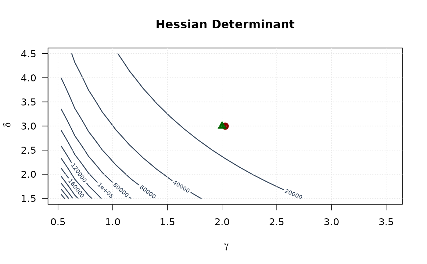
## Example 5: Curvature Visualization (Gamma vs Delta)
# Create grid around MLE
gamma_grid <- seq(mle[1] - 1.5, mle[1] + 1.5, length.out = 25)
delta_grid <- seq(mle[2] - 1.5, mle[2] + 1.5, length.out = 25)
gamma_grid <- gamma_grid[gamma_grid > 0]
delta_grid <- delta_grid[delta_grid > 0]
# Compute curvature measures
determinant_surface <- matrix(NA,
nrow = length(gamma_grid),
ncol = length(delta_grid)
)
trace_surface <- matrix(NA,
nrow = length(gamma_grid),
ncol = length(delta_grid)
)
for (i in seq_along(gamma_grid)) {
for (j in seq_along(delta_grid)) {
H <- hsbeta(c(gamma_grid[i], delta_grid[j]), data)
determinant_surface[i, j] <- det(H)
trace_surface[i, j] <- sum(diag(H))
}
}
# Plot
contour(gamma_grid, delta_grid, determinant_surface,
xlab = expression(gamma), ylab = expression(delta),
main = "Hessian Determinant", las = 1,
col = "#2E4057", lwd = 1.5, nlevels = 15
)
points(mle[1], mle[2], pch = 19, col = "#8B0000", cex = 1.5)
points(true_params[1], true_params[2], pch = 17, col = "#006400", cex = 1.5)
grid(col = "gray90")
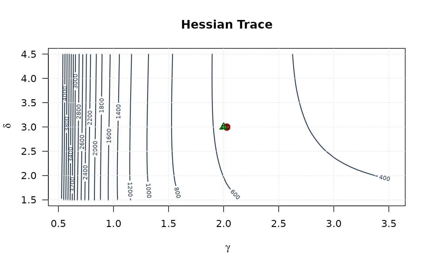
 contour(gamma_grid, delta_grid, trace_surface,
xlab = expression(gamma), ylab = expression(delta),
main = "Hessian Trace", las = 1,
col = "#2E4057", lwd = 1.5, nlevels = 15
)
points(mle[1], mle[2], pch = 19, col = "#8B0000", cex = 1.5)
points(true_params[1], true_params[2], pch = 17, col = "#006400", cex = 1.5)
grid(col = "gray90")
contour(gamma_grid, delta_grid, trace_surface,
xlab = expression(gamma), ylab = expression(delta),
main = "Hessian Trace", las = 1,
col = "#2E4057", lwd = 1.5, nlevels = 15
)
points(mle[1], mle[2], pch = 19, col = "#8B0000", cex = 1.5)
points(true_params[1], true_params[2], pch = 17, col = "#006400", cex = 1.5)
grid(col = "gray90")
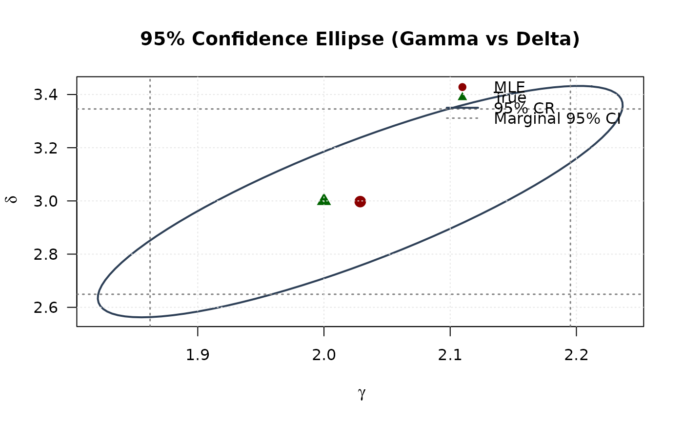
 ## Example 6: Confidence Ellipse (Gamma vs Delta)
# Extract 2x2 submatrix (full matrix in this case)
vcov_2d <- vcov_matrix
# Create confidence ellipse
theta <- seq(0, 2 * pi, length.out = 100)
chi2_val <- qchisq(0.95, df = 2)
eig_decomp <- eigen(vcov_2d)
ellipse <- matrix(NA, nrow = 100, ncol = 2)
for (i in 1:100) {
v <- c(cos(theta[i]), sin(theta[i]))
ellipse[i, ] <- mle + sqrt(chi2_val) *
(eig_decomp$vectors %*% diag(sqrt(eig_decomp$values)) %*% v)
}
# Marginal confidence intervals
se_2d <- sqrt(diag(vcov_2d))
ci_gamma <- mle[1] + c(-1, 1) * 1.96 * se_2d[1]
ci_delta <- mle[2] + c(-1, 1) * 1.96 * se_2d[2]
# Plot
plot(ellipse[, 1], ellipse[, 2],
type = "l", lwd = 2, col = "#2E4057",
xlab = expression(gamma), ylab = expression(delta),
main = "95% Confidence Ellipse (Gamma vs Delta)", las = 1
)
# Add marginal CIs
abline(v = ci_gamma, col = "#808080", lty = 3, lwd = 1.5)
abline(h = ci_delta, col = "#808080", lty = 3, lwd = 1.5)
points(mle[1], mle[2], pch = 19, col = "#8B0000", cex = 1.5)
points(true_params[1], true_params[2], pch = 17, col = "#006400", cex = 1.5)
legend("topright",
legend = c("MLE", "True", "95% CR", "Marginal 95% CI"),
col = c("#8B0000", "#006400", "#2E4057", "#808080"),
pch = c(19, 17, NA, NA),
lty = c(NA, NA, 1, 3),
lwd = c(NA, NA, 2, 1.5),
bty = "n"
)
grid(col = "gray90")
## Example 6: Confidence Ellipse (Gamma vs Delta)
# Extract 2x2 submatrix (full matrix in this case)
vcov_2d <- vcov_matrix
# Create confidence ellipse
theta <- seq(0, 2 * pi, length.out = 100)
chi2_val <- qchisq(0.95, df = 2)
eig_decomp <- eigen(vcov_2d)
ellipse <- matrix(NA, nrow = 100, ncol = 2)
for (i in 1:100) {
v <- c(cos(theta[i]), sin(theta[i]))
ellipse[i, ] <- mle + sqrt(chi2_val) *
(eig_decomp$vectors %*% diag(sqrt(eig_decomp$values)) %*% v)
}
# Marginal confidence intervals
se_2d <- sqrt(diag(vcov_2d))
ci_gamma <- mle[1] + c(-1, 1) * 1.96 * se_2d[1]
ci_delta <- mle[2] + c(-1, 1) * 1.96 * se_2d[2]
# Plot
plot(ellipse[, 1], ellipse[, 2],
type = "l", lwd = 2, col = "#2E4057",
xlab = expression(gamma), ylab = expression(delta),
main = "95% Confidence Ellipse (Gamma vs Delta)", las = 1
)
# Add marginal CIs
abline(v = ci_gamma, col = "#808080", lty = 3, lwd = 1.5)
abline(h = ci_delta, col = "#808080", lty = 3, lwd = 1.5)
points(mle[1], mle[2], pch = 19, col = "#8B0000", cex = 1.5)
points(true_params[1], true_params[2], pch = 17, col = "#006400", cex = 1.5)
legend("topright",
legend = c("MLE", "True", "95% CR", "Marginal 95% CI"),
col = c("#8B0000", "#006400", "#2E4057", "#808080"),
pch = c(19, 17, NA, NA),
lty = c(NA, NA, 1, 3),
lwd = c(NA, NA, 2, 1.5),
bty = "n"
)
grid(col = "gray90")
 # }
# }