Optimal Binning for Numerical Features using Minimum Description Length Principle

Implements the Minimum Description Length Principle (MDLP) for supervised discretization of numerical features. MDLP balances model complexity (number of bins) and data fit (information gain) through a rigorous information-theoretic framework, automatically determining the optimal number of bins without arbitrary thresholds.

Unlike heuristic methods, MDLP provides a theoretically grounded stopping criterion based on the trade-off between encoding the binning structure and encoding the data given that structure. This makes it particularly robust against overfitting in noisy datasets.

Usage

ob_numerical_mdlp(
  feature,
  target,
  min_bins = 3,
  max_bins = 5,
  bin_cutoff = 0.05,
  max_n_prebins = 20,
  convergence_threshold = 1e-06,
  max_iterations = 1000,
  laplace_smoothing = 0.5
)

Arguments

feature: Numeric vector of feature values to be binned. Missing values (NA) are automatically removed during preprocessing. Infinite values trigger a warning but are handled internally.
target: Integer vector of binary target values (must contain only 0 and 1). Must have the same length as feature.
min_bins: Minimum number of bins to generate (default: 3). Must be at least 1. If the number of unique feature values is less than min_bins, the algorithm adjusts automatically.
max_bins: Maximum number of bins to generate (default: 5). Must be greater than or equal to min_bins. Acts as a hard constraint after MDLP optimization.
bin_cutoff: Minimum fraction of total observations required in each bin (default: 0.05). Bins with frequency below this threshold are merged with adjacent bins to ensure statistical reliability. Must be in the range (0, 1).
max_n_prebins: Maximum number of pre-bins before MDLP optimization (default: 20). Higher values allow finer granularity but increase computational cost. Must be at least 2.
convergence_threshold: Convergence threshold for iterative optimization (default: 1e-6). Currently used internally for future extensions; MDLP convergence is primarily determined by the MDL cost function.
max_iterations: Maximum number of iterations for bin merging operations (default: 1000). Prevents infinite loops in pathological cases. A warning is issued if this limit is reached.
laplace_smoothing: Laplace smoothing parameter for WoE calculation (default: 0.5). Prevents division by zero and stabilizes WoE estimates in bins with zero counts for one class. Must be non-negative. Higher values increase regularization but may dilute signal in small bins.

Value

A list containing:

id: Integer vector of bin identifiers (1-based indexing).
bin: Character vector of bin intervals in the format "[lower;upper)". The first bin starts with -Inf and the last bin ends with +Inf.
woe: Numeric vector of Weight of Evidence values for each bin, computed with Laplace smoothing.
iv: Numeric vector of Information Value contributions for each bin.
count: Integer vector of total observations in each bin.
count_pos: Integer vector of positive class (target = 1) counts per bin.
count_neg: Integer vector of negative class (target = 0) counts per bin.
cutpoints: Numeric vector of cutpoints defining bin boundaries (excluding -Inf and +Inf). These are the upper bounds of bins 1 to k-1.
total_iv: Numeric scalar representing the total Information Value (sum of all bin IVs).
converged: Logical flag indicating whether the algorithm converged. Set to FALSE if max_iterations was reached during any merging phase.
iterations: Integer count of iterations performed across all optimization phases (MDL merging, rare bin merging, monotonicity enforcement).

Details

Algorithm Overview

The MDLP algorithm executes in five sequential phases:

Phase 1: Data Preparation and Validation

Input data is validated for:

Binary target (only 0 and 1 values)
Parameter consistency (min_bins <= max_bins, valid ranges)
Missing value detection (NaN/Inf are filtered out with a warning)

Feature-target pairs are sorted by feature value in ascending order, enabling efficient bin assignment via linear scan.

Phase 2: Equal-Frequency Pre-binning

Initial bins are created by dividing the sorted data into approximately equal-sized groups:

$$n_{\text{records/bin}} = \max\left(1, \left\lfloor \frac{N}{\text{max\_n\_prebins}} \right\rfloor\right)$$

This ensures each pre-bin has sufficient observations for stable entropy estimation. Bin boundaries are set to feature values at split points, with first and last boundaries at $-\infty$ and $+\infty$.

For each bin $i$, Shannon entropy is computed:

$$H(S_i) = -p_i \log_2(p_i) - q_i \log_2(q_i)$$

where $p_i = n_i^{+} / n_i$ (proportion of positives) and $q_i = 1 - p_i$. Pure bins ($p_i = 0$ or $p_i = 1$) have $H(S_i) = 0$.

Performance Note: Entropy calculation uses a precomputed lookup table for bin counts 0-100, achieving 30-50% speedup compared to runtime computation.

Phase 3: MDL-Based Greedy Merging

The core optimization minimizes the Minimum Description Length, defined as:

$$\text{MDL}(k) = L_{\text{model}}(k) + L_{\text{data}}(k)$$

where:

Model Cost: $L_{\text{model}}(k) = \log_2(k - 1)$

Encodes the number of bins. Increases logarithmically with bin count, penalizing complex models.
Data Cost: $L_{\text{data}}(k) = N \cdot H(S_{\text{total}}) - \sum_{i=1}^{k} n_i \cdot H(S_i)$

Measures unexplained uncertainty after binning. Lower values indicate better class separation.

The algorithm iteratively evaluates all $k-1$ adjacent bin pairs, computing $\text{MDL}(k-1)$ for each potential merge. The pair minimizing MDL cost is merged, continuing until:

$k = \text{min\_bins}$, or
No merge reduces MDL cost (local optimum), or
max_iterations is reached

Theoretical Guarantee (Fayyad & Irani, 1993): The MDL criterion provides a **consistent estimator** of the true discretization complexity under mild regularity conditions, unlike ad-hoc stopping rules.

Phase 4: Rare Bin Handling

Bins with frequency $n_i / N < \text{bin\_cutoff}$ are merged with adjacent bins. The merge direction (left or right) is chosen by minimizing post-merge entropy:

$$\text{direction} = \arg\min_{d \in \{\text{left}, \text{right}\}} H(S_i \cup S_{i+d})$$

This preserves class homogeneity while ensuring statistical reliability.

Phase 5: Monotonicity Enforcement (Optional)

If WoE values violate monotonicity ($\text{WoE}_i < \text{WoE}_{i-1}$), bins are iteratively merged until:

$$\text{WoE}_1 \le \text{WoE}_2 \le \cdots \le \text{WoE}_k$$

Merge decisions prioritize preserving Information Value:

$$\Delta \text{IV} = \text{IV}_i + \text{IV}_{i+1} - \text{IV}_{\text{merged}}$$

Merges proceed only if $\text{IV}_{\text{merged}} \ge 0.5 \times (\text{IV}_i + \text{IV}_{i+1})$.

Weight of Evidence Computation

WoE for bin $i$ includes Laplace smoothing to handle zero counts:

$$\text{WoE}_i = \ln\left(\frac{n_i^{+} + \alpha}{n^{+} + k\alpha} \bigg/ \frac{n_i^{-} + \alpha}{n^{-} + k\alpha}\right)$$

where $\alpha = \text{laplace\_smoothing}$ and $k$ is the number of bins.

Edge cases:

If $n_i^{+} + \alpha = n_i^{-} + \alpha = 0$: $\text{WoE}_i = 0$
If $n_i^{+} + \alpha = 0$: $\text{WoE}_i = -20$ (capped)
If $n_i^{-} + \alpha = 0$: $\text{WoE}_i = +20$ (capped)

Information Value is computed as:

$$\text{IV}_i = \left(\frac{n_i^{+}}{n^{+}} - \frac{n_i^{-}}{n^{-}}\right) \times \text{WoE}_i$$

Comparison with Other Methods

Method	Stopping Criterion	Optimality
MDLP	Information-theoretic (MDL cost)	Local optimum with theoretical guarantees
LDB	Heuristic (density minima)	No formal optimality
MBLP	Heuristic (IV loss threshold)	Greedy approximation
ChiMerge	Statistical ($\chi^2$ test)	Dependent on significance level

Computational Complexity

Sorting: $O(N \log N)$
Pre-binning: $O(N)$
MDL optimization: $O(k^3 \times I)$ where $I$ is the number of merge iterations (typically $I \approx k$)
Total: $O(N \log N + k^3 \times I)$

For typical credit scoring datasets ($N \sim 10^5$, $k \sim 5$), runtime is dominated by sorting.

References

Fayyad, U. M., & Irani, K. B. (1993). "Multi-Interval Discretization of Continuous-Valued Attributes for Classification Learning". Proceedings of the 13th International Joint Conference on Artificial Intelligence (IJCAI), pp. 1022-1027.
Rissanen, J. (1978). "Modeling by shortest data description". Automatica, 14(5), 465-471.
Shannon, C. E. (1948). "A Mathematical Theory of Communication". Bell System Technical Journal, 27(3), 379-423.
Dougherty, J., Kohavi, R., & Sahami, M. (1995). "Supervised and Unsupervised Discretization of Continuous Features". Proceedings of the 12th International Conference on Machine Learning (ICML), pp. 194-202.
Witten, I. H., Frank, E., & Hall, M. A. (2011). Data Mining: Practical Machine Learning Tools and Techniques (3rd ed.). Morgan Kaufmann.
Cerqueira, V., & Torgo, L. (2019). "Automatic Feature Engineering for Predictive Modeling of Multivariate Time Series". arXiv:1910.01344.

Author

Lopes, J. E. (algorithm implementation based on Fayyad & Irani, 1993)

Examples

# \donttest{
# Simulate overdispersed credit scoring data with noise
set.seed(2024)
n <- 10000

# Create feature with multiple regimes and noise
feature <- c(
  rnorm(3000, mean = 580, sd = 70), # High-risk cluster
  rnorm(4000, mean = 680, sd = 50), # Medium-risk cluster
  rnorm(2000, mean = 740, sd = 40), # Low-risk cluster
  runif(1000, min = 500, max = 800) # Noise (uniform distribution)
)

target <- c(
  rbinom(3000, 1, 0.30), # 30% default rate
  rbinom(4000, 1, 0.12), # 12% default rate
  rbinom(2000, 1, 0.04), # 4% default rate
  rbinom(1000, 1, 0.15) # Noisy segment
)

# Apply MDLP with default parameters
result <- ob_numerical_mdlp(
  feature = feature,
  target = target,
  min_bins = 3,
  max_bins = 5,
  bin_cutoff = 0.05,
  max_n_prebins = 20
)

# Inspect results
print(result$bin)
#> [1] "[-Inf;732.055011)"       "[732.055011;778.058805)"
#> [3] "[778.058805;+Inf)"      
print(data.frame(
  Bin = result$bin,
  WoE = round(result$woe, 4),
  IV = round(result$iv, 4),
  Count = result$count
))
#>                       Bin     WoE     IV Count
#> 1       [-Inf;732.055011)  0.1350 0.0152  8000
#> 2 [732.055011;778.058805) -0.7283 0.0618  1500
#> 3       [778.058805;+Inf) -0.7213 0.0203   500

cat(sprintf("\nTotal IV: %.4f\n", result$total_iv))
#> 
#> Total IV: 0.0973
cat(sprintf("Converged: %s\n", result$converged))
#> Converged: TRUE
cat(sprintf("Iterations: %d\n", result$iterations))
#> Iterations: 16

# Verify monotonicity
is_monotonic <- all(diff(result$woe) >= -1e-10)
cat(sprintf("WoE Monotonic: %s\n", is_monotonic))
#> WoE Monotonic: FALSE

# Compare with different Laplace smoothing
result_nosmooth <- ob_numerical_mdlp(
  feature = feature,
  target = target,
  laplace_smoothing = 0.0 # No smoothing (risky for rare bins)
)

result_highsmooth <- ob_numerical_mdlp(
  feature = feature,
  target = target,
  laplace_smoothing = 2.0 # Higher regularization
)

# Compare WoE stability
data.frame(
  Bin = seq_along(result$woe),
  WoE_default = result$woe,
  WoE_no_smooth = result_nosmooth$woe,
  WoE_high_smooth = result_highsmooth$woe
)
#>   Bin WoE_default WoE_no_smooth WoE_high_smooth
#> 1   1   0.1349518     0.1354243       0.1335385
#> 2   2  -0.7283036    -0.7310697      -0.7200885
#> 3   3  -0.7213401    -0.7310697      -0.6929202

# Visualize binning structure
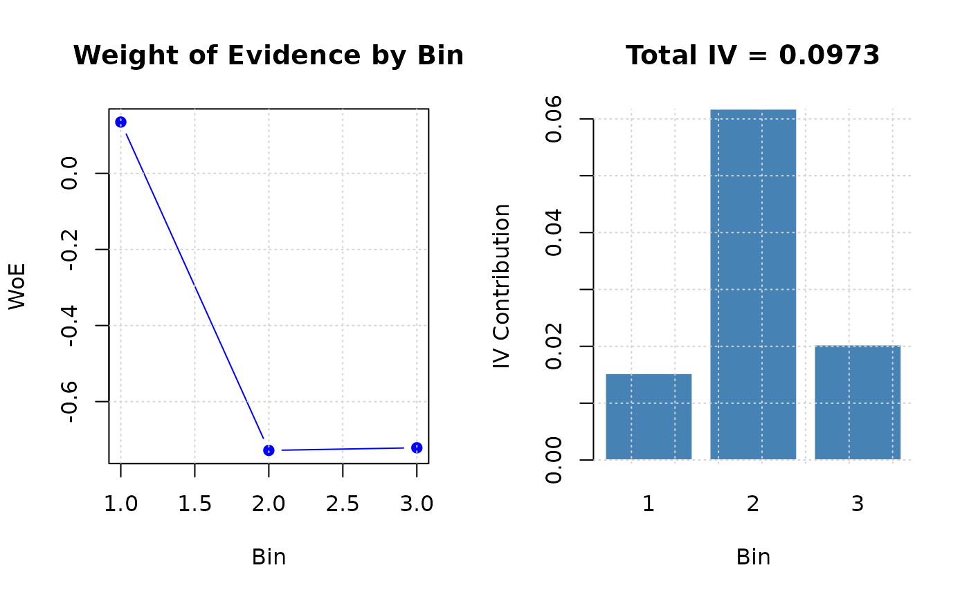
oldpar <- par(mfrow = c(1, 2))

# WoE plot
plot(result$woe,
  type = "b", col = "blue", pch = 19,
  xlab = "Bin", ylab = "WoE",
  main = "Weight of Evidence by Bin"
)
grid()

# IV contribution plot
barplot(result$iv,
  names.arg = seq_along(result$iv),
  col = "steelblue", border = "white",
  xlab = "Bin", ylab = "IV Contribution",
  main = sprintf("Total IV = %.4f", result$total_iv)
)
grid()

par(oldpar)
# }