Optimal Binning for Numerical Variables using Local Density Binning

Implements supervised discretization via Local Density Binning (LDB), a method that leverages kernel density estimation to identify natural transition regions in the feature space while optimizing the Weight of Evidence (WoE) monotonicity and Information Value (IV) for binary classification tasks.

Usage

ob_numerical_ldb(
  feature,
  target,
  min_bins = 3,
  max_bins = 5,
  bin_cutoff = 0.05,
  max_n_prebins = 20,
  enforce_monotonic = TRUE,
  convergence_threshold = 1e-06,
  max_iterations = 1000
)

Arguments

feature: Numeric vector of feature values to be binned. Missing values (NA) and infinite values are automatically filtered out during preprocessing.
target: Integer vector of binary target values (must contain only 0 and 1). Must have the same length as feature.
min_bins: Minimum number of bins to generate (default: 3). Must be at least 2.
max_bins: Maximum number of bins to generate (default: 5). Must be greater than or equal to min_bins.
bin_cutoff: Minimum fraction of total observations in each bin (default: 0.05). Bins with frequency below this threshold are merged with adjacent bins. Must be in the range [0, 1].
max_n_prebins: Maximum number of pre-bins before optimization (default: 20). Controls granularity of initial density-based discretization.
enforce_monotonic: Logical flag to enforce monotonicity in WoE values across bins (default: TRUE). When enabled, bins violating monotonicity are iteratively merged until global monotonicity is achieved.
convergence_threshold: Convergence threshold for iterative optimization (default: 1e-6). Currently used for future extensions.
max_iterations: Maximum number of iterations for merging operations (default: 1000). Prevents infinite loops in edge cases.

Value

A list containing:

id: Integer vector of bin identifiers (1-based indexing).
bin: Character vector of bin intervals in the format "(lower;upper]".
woe: Numeric vector of Weight of Evidence values for each bin.
iv: Numeric vector of Information Value contributions for each bin.
count: Integer vector of total observations in each bin.
count_pos: Integer vector of positive class (target = 1) counts per bin.
count_neg: Integer vector of negative class (target = 0) counts per bin.
event_rate: Numeric vector of event rates (proportion of positives) per bin.
cutpoints: Numeric vector of cutpoints defining bin boundaries (excluding -Inf and +Inf).
converged: Logical flag indicating whether the algorithm converged within max_iterations.
iterations: Integer count of iterations performed during optimization.
total_iv: Numeric scalar representing the total Information Value (sum of all bin IVs).
monotonicity: Character string indicating monotonicity status: "increasing", "decreasing", or "none".

Details

Algorithm Overview

The Local Density Binning (LDB) algorithm operates in four sequential phases:

Phase 1: Density-Based Pre-binning

The algorithm employs kernel density estimation (KDE) with a Gaussian kernel to identify the local density structure of the feature:

$$\hat{f}(x) = \frac{1}{nh\sqrt{2\pi}} \sum_{i=1}^{n} \exp\left[-\frac{(x - x_i)^2}{2h^2}\right]$$

where $h$ is the bandwidth computed via Silverman's rule of thumb:

$$h = 0.9 \times \min(\hat{\sigma}, \text{IQR}/1.34) \times n^{-1/5}$$

Bin boundaries are placed at local minima of $\hat{f}(x)$, which correspond to natural transition regions where density is lowest (analogous to valleys in the density landscape). This strategy ensures bins capture homogeneous subpopulations.

Phase 2: Weight of Evidence Computation

For each bin $i$, the WoE quantifies the log-ratio of positive to negative class distributions, adjusted with Laplace smoothing ($\alpha = 0.5$) to prevent division by zero:

$$\text{WoE}_i = \ln\left(\frac{\text{DistGood}_i}{\text{DistBad}_i}\right)$$

where:

$$\text{DistGood}_i = \frac{n_{i}^{+} + \alpha}{n^{+} + K\alpha}, \quad \text{DistBad}_i = \frac{n_{i}^{-} + \alpha}{n^{-} + K\alpha}$$

and $K$ is the total number of bins. The Information Value for bin $i$ is:

$$\text{IV}_i = (\text{DistGood}_i - \text{DistBad}_i) \times \text{WoE}_i$$

Total IV aggregates discriminatory power: $\text{IV}_{\text{total}} = \sum_{i=1}^{K} \text{IV}_i$.

Phase 3: Monotonicity Enforcement

When enforce_monotonic = TRUE, the algorithm ensures WoE values are monotonic with respect to bin order. The direction (increasing/decreasing) is determined via Pearson correlation between bin indices and WoE values. Bins violating monotonicity are iteratively merged using the merge strategy described in Phase 4, continuing until global monotonicity is achieved or min_bins is reached.

This approach is rooted in isotonic regression principles (Robertson et al., 1988), ensuring the scorecard maintains a consistent logical relationship between feature values and credit risk.

Phase 4: Adaptive Bin Merging

Two merging criteria are applied sequentially:

Frequency-based merging: Bins with total count below bin_cutoff $\times n$ are merged with the adjacent bin having the most similar event rate (minimizing heterogeneity). If event rates are equivalent, the merge that preserves higher IV is preferred.
Cardinality reduction: If the number of bins exceeds max_bins, the pair of adjacent bins minimizing IV loss when merged is identified via: $$\Delta \text{IV}_{i,i+1} = \text{IV}_i + \text{IV}_{i+1} - \text{IV}_{\text{merged}}$$ This greedy optimization continues until $K \le$ max_bins.

Theoretical Foundations

Kernel Density Estimation: The bandwidth selection follows Silverman (1986, Chapter 3), balancing bias-variance tradeoff for univariate density estimation.
Weight of Evidence: Siddiqi (2006) formalizes WoE/IV as measures of predictive strength in credit scoring, with IV thresholds: $< 0.02$ (unpredictive), 0.02-0.1 (weak), 0.1-0.3 (medium), 0.3-0.5 (strong), $> 0.5$ (suspect overfitting).
Supervised Discretization: García et al. (2013) categorize LDB within "static" supervised methods that do not require iterative feedback from the model, unlike dynamic methods (e.g., ChiMerge).

Computational Complexity

KDE computation: $O(n^2)$ for naive implementation (each of $n$ points evaluates $n$ kernel terms).
Binary search for bin assignment: $O(n \log K)$ where $K$ is the number of bins.
Merge iterations: $O(K^2 \times \text{max\_iterations})$ in worst case.

For large datasets ($n > 10^5$), the KDE phase dominates runtime.

References

Silverman, B. W. (1986). Density Estimation for Statistics and Data Analysis. Chapman and Hall/CRC.
Siddiqi, N. (2006). Credit Risk Scorecards: Developing and Implementing Intelligent Credit Scoring. Wiley.
Dougherty, J., Kohavi, R., & Sahami, M. (1995). "Supervised and Unsupervised Discretization of Continuous Features". Proceedings of the 12th International Conference on Machine Learning, pp. 194-202.
Robertson, T., Wright, F. T., & Dykstra, R. L. (1988). Order Restricted Statistical Inference. Wiley.
García, S., Luengo, J., Sáez, J. A., López, V., & Herrera, F. (2013). "A Survey of Discretization Techniques: Taxonomy and Empirical Analysis in Supervised Learning". IEEE Transactions on Knowledge and Data Engineering, 25(4), 734-750.

Author

Lopes, J. E. (implemented algorithm)

Examples

# \donttest{
# Simulate credit scoring data
set.seed(42)
n <- 10000
feature <- c(
  rnorm(3000, mean = 600, sd = 50), # Low-risk segment
  rnorm(4000, mean = 700, sd = 40), # Medium-risk segment
  rnorm(3000, mean = 750, sd = 30) # High-risk segment
)
target <- c(
  rbinom(3000, 1, 0.15), # 15% default rate
  rbinom(4000, 1, 0.08), # 8% default rate
  rbinom(3000, 1, 0.03) # 3% default rate
)

# Apply LDB with monotonicity enforcement
result <- ob_numerical_ldb(
  feature = feature,
  target = target,
  min_bins = 3,
  max_bins = 5,
  bin_cutoff = 0.05,
  max_n_prebins = 20,
  enforce_monotonic = TRUE
)

# Inspect binning quality
print(result$total_iv) # Should be > 0.1 for predictive features
#> [1] 0.1914946
print(result$monotonicity) # Should indicate direction
#> [1] "decreasing"

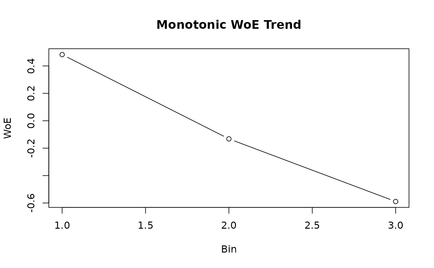
# Visualize WoE pattern
plot(result$woe,
  type = "b", xlab = "Bin", ylab = "WoE",
  main = "Monotonic WoE Trend"
)


# Generate scorecard transformation
bin_mapping <- data.frame(
  bin = result$bin,
  woe = result$woe,
  iv = result$iv
)
print(bin_mapping)
#>                       bin        woe          iv
#> 1       (-Inf;660.733735]  0.4827072 0.094830755
#> 2 (660.733735;726.780204] -0.1320751 0.005514779
#> 3       (726.780204;+Inf] -0.5891944 0.091149091
# }