Categorical Optimal Binning with Fisher’s Exact Test

Performs supervised optimal binning of a categorical predictor versus a binary target by iteratively merging the most similar adjacent bins according to Fisher’s Exact Test. The routine returns monotonic Weight of Evidence (WoE) values and the associated Information Value (IV), both key metrics in credit‑scoring, churn prediction and other binary‑response models.

Usage

optimal_binning_categorical_fetb(
  target,
  feature,
  min_bins = 3L,
  max_bins = 5L,
  bin_cutoff = 0.05,
  max_n_prebins = 20L,
  convergence_threshold = 1e-06,
  max_iterations = 1000L,
  bin_separator = "%;%"
)

Arguments

target

integer vector of 0/1 values (length \(N\)).

feature

character vector of categories (length \(N\)).

min_bins

Minimum number of final bins. Default is 3.

max_bins

Maximum number of final bins. Default is 5.

bin_cutoff

Relative frequency threshold below which categories are folded into the rare‑bin (default 0.05).

max_n_prebins

Reserved for future use (ignored internally).

convergence_threshold

Absolute tolerance for the change in total IV required to declare convergence (default 0.0000001).

max_iterations

Safety cap for merge iterations (default 1000).

bin_separator

String used to concatenate category labels in the output.

Value

A list with components

• id – numeric id of each resulting bin

• bin – concatenated category labels

• woe, iv – WoE and IV per bin

• count, count_pos, count_neg – bin counts

• converged – logical flag

• iterations – number of merge iterations

Details

Algorithm outline
Let \(X \in \{\mathcal{C}_1,\dots,\mathcal{C}_K\}\) be a categorical feature and \(Y\in\{0,1\}\) the target. For each category \(\mathcal{C}_k\) compute the contingency table $$ \begin{array}{c|cc} & Y=1 & Y=0 \\ \hline X=\mathcal{C}_k & a_k & b_k \end{array}$$ with \(a_k+b_k=n_k\). Rare categories where \(n_k < \textrm{cutoff}\times N\) are grouped into a “rare” bin. The remaining categories start as singleton bins ordered by their WoE: $$\mathrm{WoE}_k = \log\left(\frac{a_k/T_1}{b_k/T_0}\right)$$ where \(T_1=\sum_k a_k,\; T_0=\sum_k b_k\).

At every iteration the two adjacent bins \(i,i+1\) that maximise the two‑tail Fisher p‑value $$p_{i,i+1} = P\!\left( \begin{array}{c|cc} & Y=1 & Y=0\\\hline \text{bin }i & a_i & b_i\\ \text{bin }i+1 & a_{i+1}& b_{i+1} \end{array} \right)$$ are merged. The process stops when either \(\#\text{bins}\le\texttt{max\_bins}\) or the change in global IV, $$\mathrm{IV}= \sum_{\text{bins}} (\tfrac{a}{T_1}-\tfrac{b}{T_0}) \log\!\left(\tfrac{a\,T_0}{b\,T_1}\right)$$ is below convergence_threshold. After each merge a local monotonicity enforcement step guarantees \(\mathrm{WoE}_1\le\cdots\le\mathrm{WoE}_m\) (or the reverse).

Complexity

• Counting pass: \(O(N)\) time and \(O(K)\) memory.

• Merging loop: worst‑case \(O(B^2)\) time where \(B\le K\) is the initial number of bins; in practice \(B\ll N\) and the loop is very fast.

Overall complexity is \(O(N + B^2)\) time and \(O(K)\) memory.

Statistical background
The use of Fisher’s Exact Test provides an exact significance measure for 2×2 tables, ensuring the merged bins are those whose class proportions do not differ significantly. Monotone WoE facilitates downstream monotonic logistic regression or scorecard scaling.

References

Fisher, R. A. (1922). On the interpretation of \(X^2\) from contingency tables, and the calculation of P. Journal of the Royal Statistical Society, 85, 87‑94.
Hosmer, D. W., & Lemeshow, S. (2000). Applied Logistic Regression (2nd ed.). Wiley.
Navas‑Palencia, G. (2019). optbinning: Optimal Binning in Python – documentation v0.19.
Freeman, J. V., & Campbell, M. J. (2007). The analysis of categorical data: Fisher’s exact test. Significance.
Siddiqi, N. (2012). Credit Risk Scorecards: Developing and Implementing Intelligent Credit Scoring. Wiley.

Author

Lopes, J. E.

Examples

# \donttest{
## simulated example -------------------------------------------------
set.seed(42)
n        <- 1000
target   <- rbinom(n, 1, 0.3)                 # 30 % positives
cats     <- LETTERS[1:6]
probs    <- c(0.25, 0.20, 0.18, 0.15, 0.12, 0.10)
feature  <- sample(cats, n, TRUE, probs)      # imbalanced categories

res <- optimal_binning_categorical_fetb(
  target, feature,
  min_bins = 2, max_bins = 4,
  bin_cutoff = 0.02, bin_separator = "|"
)

str(res)
#> List of 9
#>  $ id        : num [1:4] 1 2 3 4
#>  $ bin       : chr [1:4] "F|D" "B" "A" "E|C"
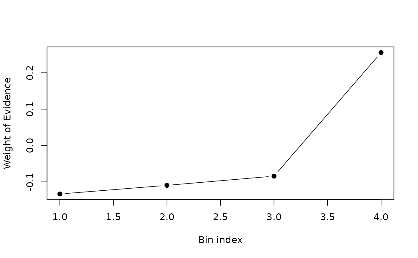
#>  $ woe       : num [1:4] -0.1333 -0.1095 -0.0842 0.2556
#>  $ iv        : num [1:4] 0.00454 0.00225 0.00182 0.01948
#>  $ count     : int [1:4] 263 192 261 284
#>  $ count_pos : int [1:4] 70 52 72 99
#>  $ count_neg : int [1:4] 193 140 189 185
#>  $ converged : logi TRUE
#>  $ iterations: int 2

## inspect WoE curve
plot(res$woe, type = "b", pch = 19,
     xlab = "Bin index", ylab = "Weight of Evidence")

# }