CDF of the Beta Distribution (gamma, delta+1 Parameterization)

Computes the cumulative distribution function (CDF), \(F(q) = P(X \le q)\), for the standard Beta distribution, using a parameterization common in generalized distribution families. The distribution is parameterized by gamma (\(\gamma\)) and delta (\(\delta\)), corresponding to the standard Beta distribution with shape parameters shape1 = gamma and shape2 = delta + 1.

Usage

pbeta_(q, gamma, delta, lower_tail = TRUE, log_p = FALSE)

Arguments

q: Vector of quantiles (values generally between 0 and 1).
gamma: First shape parameter (shape1), \(\gamma > 0\). Can be a scalar or a vector. Default: 1.0.
delta: Second shape parameter is delta + 1 (shape2), requires \(\delta \ge 0\) so that shape2 >= 1. Can be a scalar or a vector. Default: 0.0 (leading to shape2 = 1).
lower_tail: Logical; if TRUE (default), probabilities are \(P(X \le q)\), otherwise, \(P(X > q)\).
log_p: Logical; if TRUE, probabilities \(p\) are given as \(\log(p)\). Default: FALSE.

Value

A vector of probabilities, \(F(q)\), or their logarithms/complements depending on lower_tail and log_p. The length of the result is determined by the recycling rule applied to the arguments (q, gamma, delta). Returns 0 (or -Inf if log_p = TRUE) for q <= 0 and 1 (or 0 if log_p = TRUE) for q >= 1. Returns NaN for invalid parameters.

Details

This function computes the CDF of a Beta distribution with parameters shape1 = gamma and shape2 = delta + 1. It is equivalent to calling stats::pbeta(q, shape1 = gamma, shape2 = delta + 1, lower.tail = lower_tail, log.p = log_p).

This distribution arises as a special case of the five-parameter Generalized Kumaraswamy (GKw) distribution (pgkw) obtained by setting \(\alpha = 1\), \(\beta = 1\), and \(\lambda = 1\). It is therefore also equivalent to the McDonald (Mc)/Beta Power distribution (pmc) with \(\lambda = 1\).

The function likely calls R's underlying pbeta function but ensures consistent parameter recycling and handling within the C++ environment, matching the style of other functions in the related families.

References

Johnson, N. L., Kotz, S., & Balakrishnan, N. (1995). Continuous Univariate Distributions, Volume 2 (2nd ed.). Wiley.

Cordeiro, G. M., & de Castro, M. (2011). A new family of generalized distributions. Journal of Statistical Computation and Simulation,

Author

Lopes, J. E.

Examples

# \donttest{
# Example values
q_vals <- c(0.2, 0.5, 0.8)
gamma_par <- 2.0 # Corresponds to shape1
delta_par <- 3.0 # Corresponds to shape2 - 1
shape1 <- gamma_par
shape2 <- delta_par + 1

# Calculate CDF using pbeta_
probs <- pbeta_(q_vals, gamma_par, delta_par)
print(probs)
#> [1] 0.26272 0.81250 0.99328

# Compare with stats::pbeta
probs_stats <- stats::pbeta(q_vals, shape1 = shape1, shape2 = shape2)
print(paste("Max difference vs stats::pbeta:", max(abs(probs - probs_stats))))
#> [1] "Max difference vs stats::pbeta: 0"

# Compare with pgkw setting alpha=1, beta=1, lambda=1
probs_gkw <- pgkw(q_vals, alpha = 1.0, beta = 1.0, gamma = gamma_par,
                  delta = delta_par, lambda = 1.0)
print(paste("Max difference vs pgkw:", max(abs(probs - probs_gkw))))
#> [1] "Max difference vs pgkw: 1.11022302462516e-16"

# Compare with pmc setting lambda=1
probs_mc <- pmc(q_vals, gamma = gamma_par, delta = delta_par, lambda = 1.0)
print(paste("Max difference vs pmc:", max(abs(probs - probs_mc))))
#> [1] "Max difference vs pmc: 0"

# Calculate upper tail P(X > q)
probs_upper <- pbeta_(q_vals, gamma_par, delta_par, lower_tail = FALSE)
print(probs_upper)
#> [1] 0.73728 0.18750 0.00672
print(stats::pbeta(q_vals, shape1, shape2, lower.tail = FALSE))
#> [1] 0.73728 0.18750 0.00672

# Calculate log CDF
log_probs <- pbeta_(q_vals, gamma_par, delta_par, log_p = TRUE)
print(log_probs)
#> [1] -1.336666453 -0.207639365 -0.006742681
print(stats::pbeta(q_vals, shape1, shape2, log.p = TRUE))
#> [1] -1.336666453 -0.207639365 -0.006742681

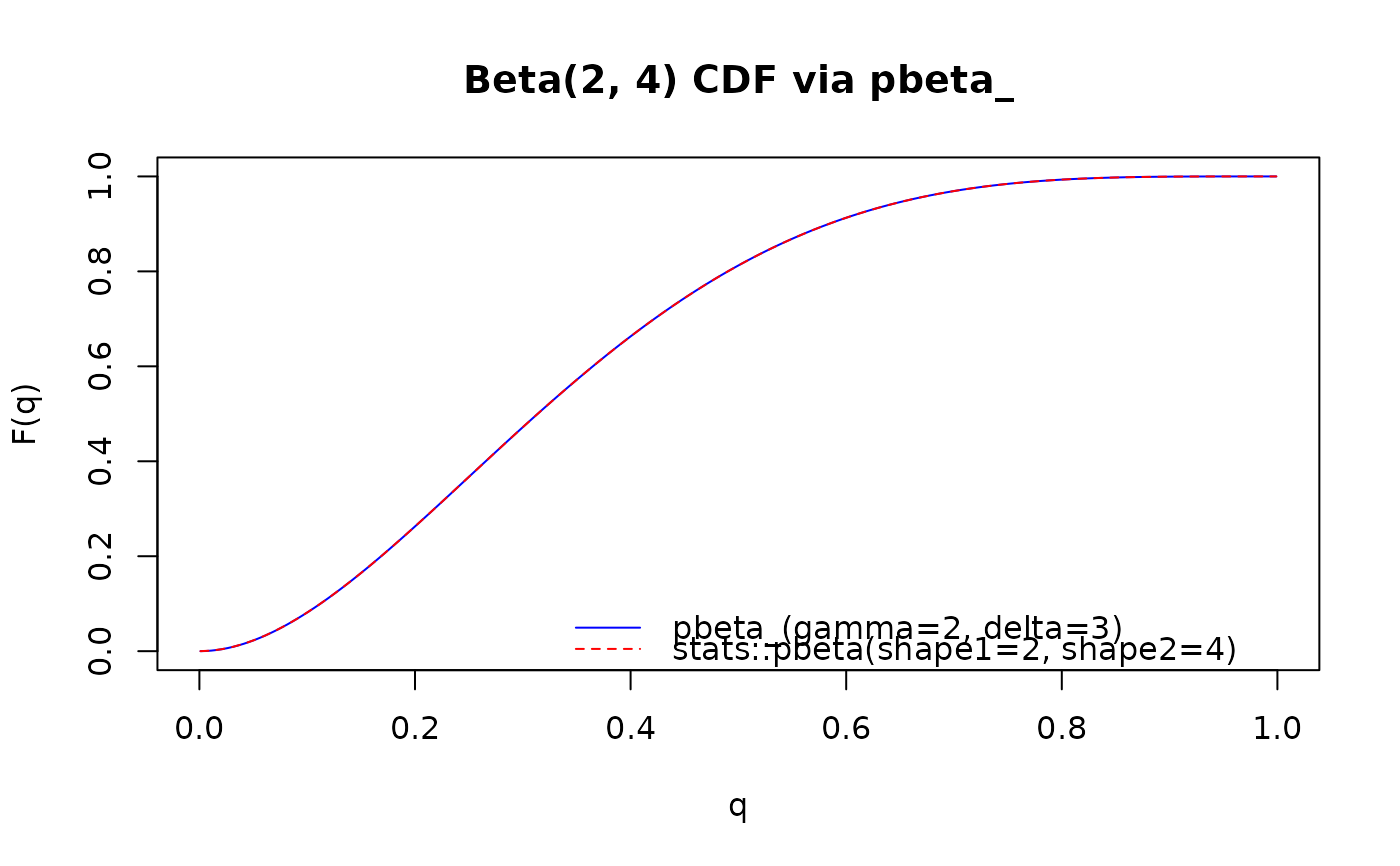
# Plot the CDF
curve_q <- seq(0.001, 0.999, length.out = 200)
curve_p <- pbeta_(curve_q, gamma = 2, delta = 3) # Beta(2, 4)
plot(curve_q, curve_p, type = "l", main = "Beta(2, 4) CDF via pbeta_",
     xlab = "q", ylab = "F(q)", col = "blue")
curve(stats::pbeta(x, 2, 4), add=TRUE, col="red", lty=2)
legend("bottomright", legend=c("pbeta_(gamma=2, delta=3)", "stats::pbeta(shape1=2, shape2=4)"),
       col=c("blue", "red"), lty=c(1,2), bty="n")


# }